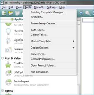
After the simulations have been setup, it is now time to run the simulation. To run the simulation click on the Run (

) button on the MicroFlo toolbar. For internal simulation it is accessible when you are at room level of decomposition. For external simulation it is available at model level of decomposition. Alternatively you can also access this via Menu -> Tools -> Run Simulation.
Figure 10-1: Run Simulation
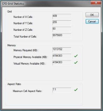
Clicking the run button will bring you to the grid statistics box. This has already been covered in
section 6.3.5.
Figure 10-2: Grid Statistics
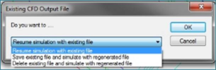
If you have run a previous simulation, it will prompt you about it.
Figure 10-3: Previous Simulation
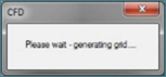
You can select one of the three options to proceed. Proceeding will generate the grid with a prompt telling you it is doing so.
Figure 10-4: Generating Grid
MicroFlo Monitor
Figure 10-5 shows the MicroFlo Monitor window.
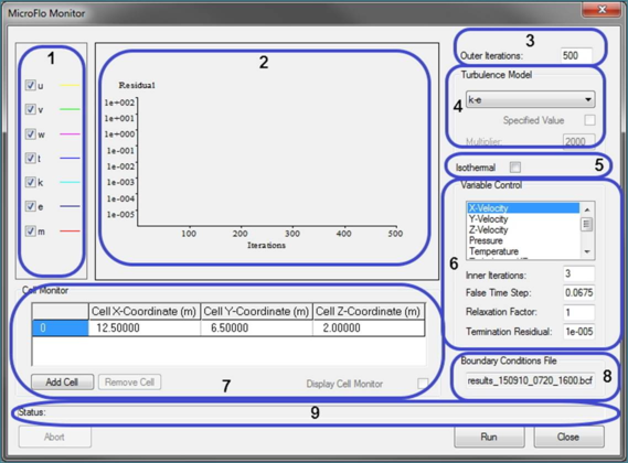
Figure 10-5: MicroFlo Monitor
The MicroFlo Monitor is divided into 8 parts as shown in the figure above
1. Legend: This legend shows the colour of the lines plotted for the residuals for the various variables. The variables are u (X-velocity), v (Y-velocity), w (Z-velocity), t (Temperature), k (Turbulent Kinetic Energy), e (Rate of dissipation of turbulent kinetic energy) and m (mass continuity).
2. Residual Plot: This is the area of the MicroFlo monitor where the residuals are plotted. Residual, in simplest terms, is the difference between the value calculated in the current outer iteration and the previous outer iteration. Convergence is achieved when the residuals falls to zero. Due to the numerical approximations involved, the residual will never become zero but fall to a value as close to zero as possible.
3. Outer Iterations: This is the number of iterations for which the solution is recalculated for.
4. Turbulence Model: This is same as explained in
section 5.1. It is provided here as a quick way of switching the turbulence model for troubleshooting.
5. Isothermal: This is the option for switching the energy solver ON/OFF. For external simulation, this box will be ticked ON and greyed out as the simulation is isothermal only.
6. Variable Control: This allows the user to define the rules for controlling the convergence of each individual variables. Not all of these are relevant to every variable being solved for. The options are:
a. Inner Iterations: This is the number of times the variable will be recalculated for each outer iteration.
b. False Time Step: This is a characteristic input of the formulation used by the solver. It ensures that any variable does not traverse more than the length of the smallest cell in the grid to ensure the correct physics is captured.
c. Relaxation Factor: This calculates how much is the solution in this outer iteration based on the solution in the previous outer iteration. Value of 1 indicates that a fresh solution is being calculated every outer iteration. Lowering the value increases the dependence of solution of this outer iteration on the previous outer iteration till value reduces to 0.
d. Termination Residual: This lowest value to which the residual of that variable is allowed to reduce to.
7. Cell Monitor: We will discuss more about this in
section 10.2.
8. Boundary Condition File: This shows the name of the boundary condition file which was used to import the data for that internal simulation. It should generally show a blank if boundary conditions have not been imported. It sometimes shows a value if you happen to run a simulation where boundary conditions have not been imported is run immediately after a simulation where boundary conditions have been imported.
9. Status bar: shows whether simulation is running or completed.
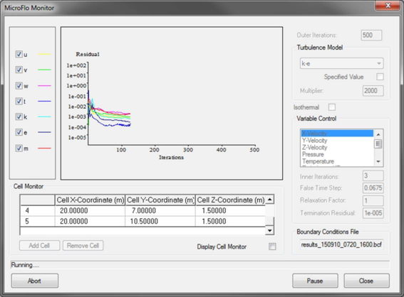
Figure 10-6 below shows how the MicroFlo Monitor looks while the simulation is running.
Figure 10-6: MicroFlo Monitor - simulation running
The simulation can be aborted by clicking on the ‘Abort’ button at the bottom. This will delete all the results and reset the simulation.
To view the results during the simulation, click on ‘Pause’ to pause the simulation. ‘Close’ the window. Then go to the MicroFlo viewer to look at the results. To resume, close the MicroFlo Viewer and click on ‘Run’. After the grid statistics you will be prompted by the dialogue seen in figure 10-3. Select appropriate option to resume the simulation.
If the simulation converges based on the convergence criteria, the residuals will slowly reduce to the level input and the status bar will say ‘Run Completed’.
If the residuals plummet to zero suddenly, then it means the solution has diverged and the simulation setup needs to be reviewed. More about this in the
Troubleshooting Section at the end.
Cell Monitors
Cell Monitors are used to record the values of various variables at locations of interest. They may also be used to gauge the convergence of the model. Since it records the values at each iteration, convergence can be assumed if the values of variables stop changing over a large number of iterations.
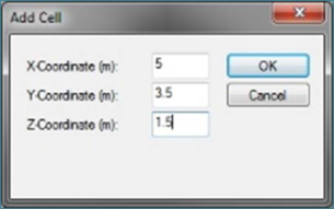
To add cell monitors, just click on the ‘Add Cell’ button underneath the list seen in section 6 of figure 10-5. It will bring the ‘Add Cell’ dialogue box.
Figure 10-7: Add Cell
Enter the coordinates of the location of interest within the appropriate boxes. Ensure that point lies within the room(s) for which analysis is being carried out. Click Ok to add the point. You can add many points like this.
Once added, you can remove the cell by selecting the point in the list and clicking ‘Remove Cell’ button. This button is activated only when more than one cell has been added. At least one cell has to be present for the simulation.
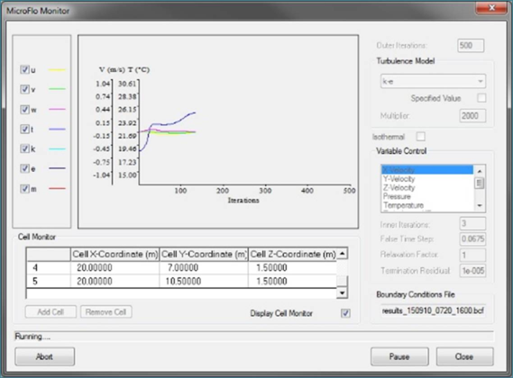
The progress of the cell monitors can be seen only when the simulation is running by clicking the check box for ‘Display Cell Monitor’.
Figure 10-8: MicroFlo Monitor: Display Cell Monitor
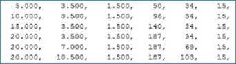
Once the simulation has been completed, you may want to read the data from the cell monitors. The results are stored in this location: project folder -> cfd -> cell.’ To find the file name corresponding to the cell, you can open the ‘.cel’ file in a text editor. It will look something like this:
Figure 10-9: Contents of ‘.cel’ file
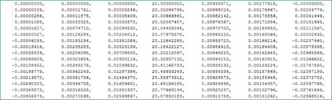
So here, the data for the cell at location (5, 3.5, 1 5) will be stored in file ‘50_34_15.log’ file in the cell folder. The data will look something like this:
Figure 10-10: Contents of the cell monitor log
The data is divided into 7 columns. In order they are x component of velocity, y component of velocity, z-component of velocity, temperature, turbulent kinetic energy, rate of dissipation of turbulent kinetic energy and local mass flow. The last variable is meaningless on its own as mass continuity is a global measure. Each line of the data corresponds to one outer iteration. After convergence, the data of relevance is the data on the last line of the log file which corresponds to the final outer iteration.