The MicroFlo viewer is the post-processing tool for MicroFlo simulations –both internal and external. It can be accessed by pressing the MicroFlo Viewer (

) button on the MicroFlo toolbar.
MicroFlo Viewer Window
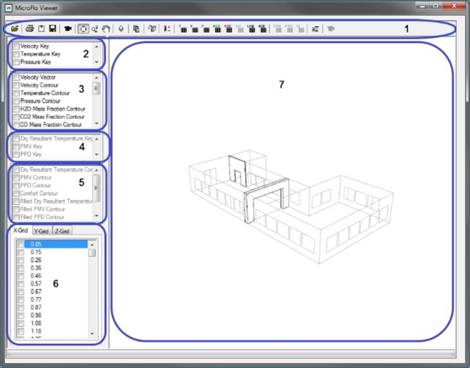
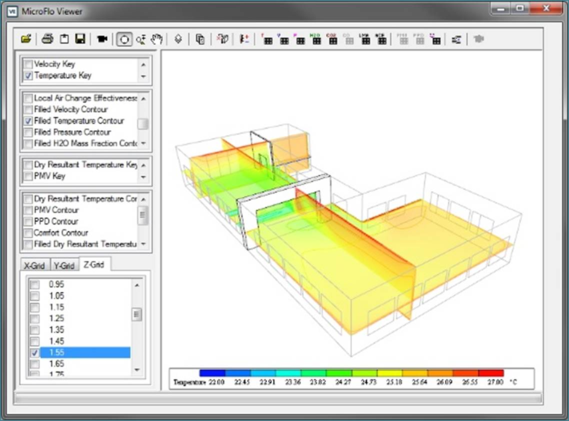
The basic layout of the MicroFlo Viewer Window is as seen in figure 11-1.
Figure 11-1: MicroFlo Viewer Window
1. MicroFlo Toolbar: This contains the buttons for basic functionality of the MicroFlo viewer.
2. List of keys of primary variables calculated during the simulation available for display by selecting one at a time.
3. List of the various types slice display options.
4. List of keys of the variables calculated in the comfort calculations
5. List of the various types slice display options for the comfort variables
6. List of available slices for display. These lie at cell centres of the cells of the grid.
7. Model window showing the results
MicroFlo Viewer Toolbar
Figure 11-2: MicroFlo Toolbar
1. Open File: Open results of a previously saved simulation file (.cdf)
2. Print: Print the view of results as displayed in the model window
3. Copy to Clipboard: Copy the contents of the model window view to the windows clipboard
4. Save image to file: Save the model view as a bitmap file
5. Create AVI: Opens the dialogue to capture video
6. Orbit: Rotates the model
7. Zoom: Zoom in and out of the model
8. Pan: Pan across the model
9. Open GL Information: Displays details on the graphics processing unit being used by the VE.
10. Display Settings: Opens the dialogue for the various settings for the MicroFlo Viewer
11. Remove all slices from display: Deletes all the slices currently on display and clears the window
12. Thermal Comfort: Opens the dialogue for the thermal comfort parameters
13. Temperature surfaces: Plots the iso surfaces of temperature
14. Velocity surfaces: Plots the iso surfaces of velocity
15. Pressure surfaces: Plots the iso surfaces of pressure
16. H2O Surfaces: Plots the iso surfaces of water vapour
17. CO2 Surfaces: Plots the iso surfaces of carbon dioxide
18. CO Surfaces: Plots the iso surfaces of carbon monoxide
19. LMA Surfaces: Plots the iso surfaces of local mean age of air
20. ACE Surfaces: Plots the iso surfaces of local air change effectiveness
21. PMV Surfaces: Plots the iso surfaces of predicted mean value
22. PPD Surfaces: Plots the iso surfaces of percentage of people dissatisfied
23. Comfort: Plots the iso surfaces of comfort parameter
24. Particle Tracking: Enables the particle tracking view in the model
25. Cancel AVI: Abort the creation of video
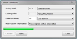
Thermal Comfort Calculator
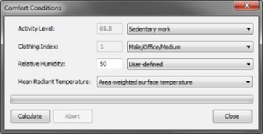
The thermal comfort calculator is activated by pressing the Thermal Comfort button on the MicroFlo Viewer Toolbar as noted in the previous section.
Figure 11-3: Comfort Conditions
The various options are:
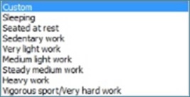
1. Activity Level: This is the type of activity the occupants of the room are expected to be carrying out. The various option are:
Figure 11-4: Options for activity level
Each option will set the appropriate activity level within the room. Using the ‘Custom’ option will allow the user to directly input the number.
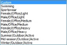
2. Clothing Index: This is the type of clothing that the occupants in the room are generally expected to be attired in. The various options are:
Figure 11-5: Options for clothing index
As before, some combinations are available as presets while any particular values can be entered by choosing the ‘Custom’ option.
3. Relative humidity: You have an option between user defined and program calculated. The program calculated option is used when the inputs related to water vapour have been specified in the simulation setup (boundary conditions and sources). In this case the relative humidity is calculated at each grid cell based on local values of temperature and moisture content. In case inputs are not provided, a global value can be applied to all cells by choosing the user-defined option.
4. Mean Radiant Temperature: The user can either choose to calculate the mean radiant temperature as the area weighted average of surface temperature or calculate it at each cell based on numerical integration.
After you click OK, the necessary parameters will be calculated.
Figure 11-6: Comfort Condition - calculating
Notes:
1. These results are very relative to the input and can produce different results for any variation for same set of results of the MicroFlo simulations
2. The results of these calculations are only stored temporarily until the MicroFlo Viewer remains open. Closing the viewer will erase the results and will have to be recalculated when the MicroFlo viewer is opened again.
3. These calculations are not available for isothermal simulation.
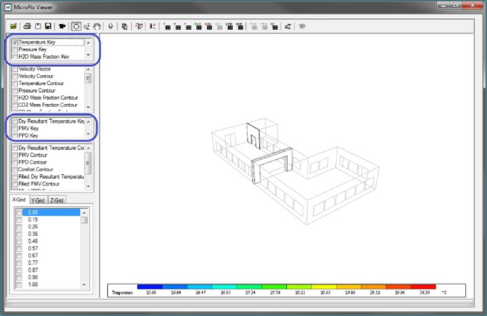
Slices
Following steps are to be followed to display contours on slices:
1. Select the appropriate key for the variable you want to display from the list of the keys.
Figure 11-7: Select the key
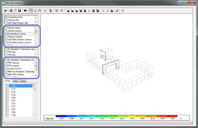
2. Select the corresponding contour from the list of contours. There are two types of contours available – line contours and filled contours. These can be combined by selecting both simultaneously.
Figure 11-8: Select the type of contour
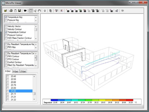
3. Final step is to click on one of the planes in the list of planes. You can scroll through these by simply clicking through the list in either of the X, Y or Z grid planes. To keep one or more planes on continuously in view, you can click the button in front of the plane. Following figures show various options for display
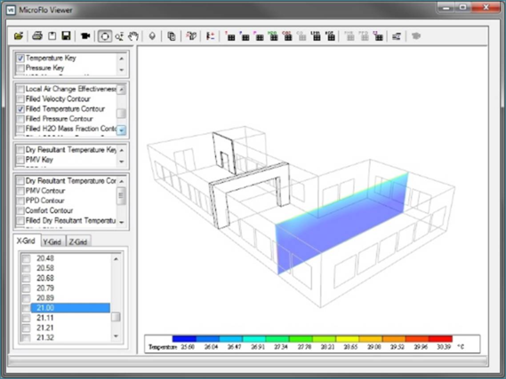
Figure 11-9: Line contours
Figure 11-10: Filled contours
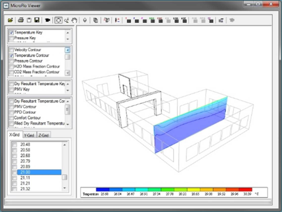
Figure 11-11: Line + filled contours
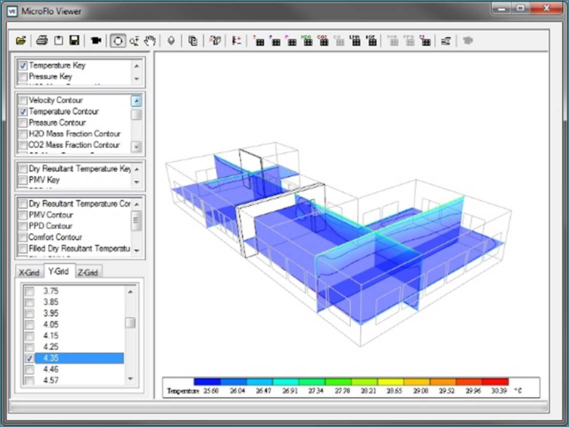
Figure 11-12: Multiple slices in display
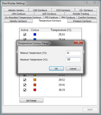
4. To change the scale of the colours, go to Display Settings and select the appropriate tab. On that tab select ‘Set Range’ to change the scale of results. Click apply after you are done. The results will change the way they are displayed. The default scale goes from the lowest to the highest recorded value of that variable.
Figure 11-13: Set new range
Figure 11-14: Results with change in scale
5. To clear the slices from display, click on ‘Remove All Slices’ button on the toolbar. This will deselect all slices in the list reset the view to the first slice in the list currently highlighted.
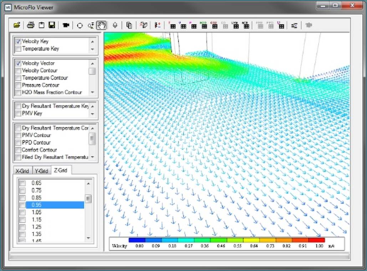
Velocity Vectors
Velocity vectors can also be displayed for velocity. These are basically arrows at the cell centres of the plane being displayed with the arrows pointing in direction of the velocity vector at that cell centre. To display the velocity vectors, follow similar procedure to above. Only changes are to select ‘Velocity Key’ and the ‘Velocity vector’ options
Figure 11-15: Velocity vectors
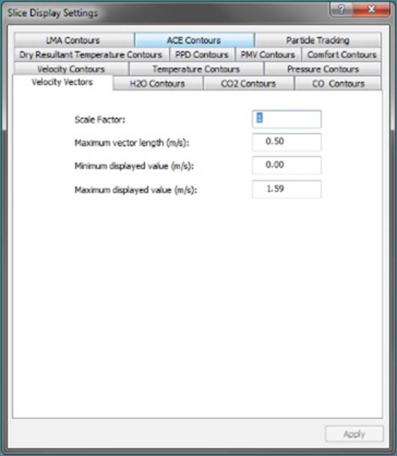
The display of velocity vectors can be changed through the ‘Velocity Vectors’ tab in the display settings.
Figure 11-16: Velocity Vectors: Slice Display Settings
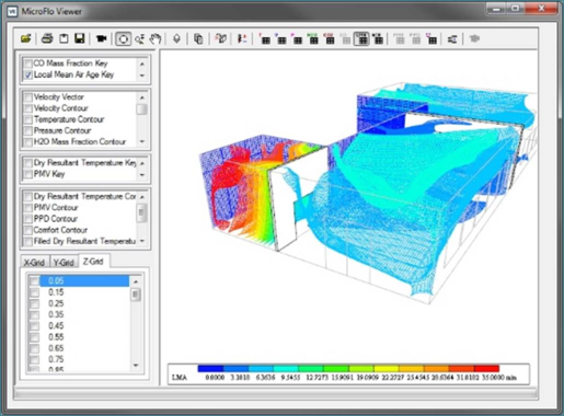
Iso-surfaces
Iso-surfaces are three dimensional contours of the variable selected. They are plotted for the entire domain based on the range of the variable as set in the display settings. To plot the iso-surface, simply select the appropriate key in the list and click on the required button the toolbar.
Figure 11-17: Iso-surfaces
Particle Tracking
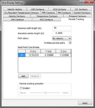
Particle tracking allows the user to visualise the path a particle would take beginning from a certain initial position. This initial position is called as a seed point. The initial settings for particle tracking are available in the ‘Particle Tracking’ tab of the ‘Display Settings’.
Figure 11-18: Particle Tracking Settings
1. Maximum Path length (m): maximum length of the path of the particle movement that you want displayed.
2. Animation marker length (m): When animation is turned on, the path is animated in form of a dash that moves along the curve. This property controls the length of this animation marker.
3. Path Colour: User has an option to colour it by velocity or temperature
4. Anti-alias particle paths: Use advanced GPU capabilities for display of the path
5. Seed Point coordinates: Enter the coordinates of the points you want the particle paths to begin from. The points have to lie inside the domain.
6. Particle tracking animation: The user can turn the animation On/Off. After it has been turned ON, the user can use the slider the increase or decrease the speed of animation.
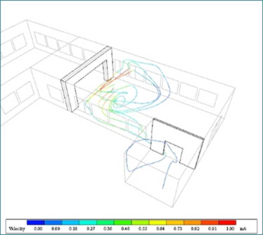
Figure 11-19: Particle tracks
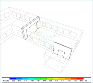
Figure 11-20: Animated particle tracks
Saving results
The results of the simulations can be saved in two ways.
Images
Make sure you have setup the scene as needed. There are three ways you save the results as images
1. Capture a screenshot of the model window.
2. Save it as a bitmap image by clicking on ‘Save’ on the toolbar.
3. Copy the current scene as an image to the clipboard by clicking on ‘Copy to Clipboard’ button on the toolbar. You can then paste the image into the software of your choice for further saving/editing.
Videos
You can also create a video of the results. To start creating a video pressure the ‘Create AVI’ button on the toolbar.
Following that there are three types of videos you can produce:
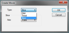
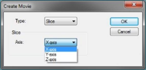
Slice
In this type of video, the viewer will record a video by displaying each slice in certain direction. Each frame of the video corresponds to one slice. Before you can do this, ensure that at least one contour type has been selected to display.
Figure 11-21: Create Movie: Slice
Then select the direction you want to traverse through.
Figure 11-22: Slice: Select direction
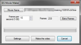
Clicking OK will capture each slice as an image in the memory and will bring up the IES Movie Maker dialog box.
Figure 11-23: IES Movie Maker
We will see more about this after we have looked at different video types.
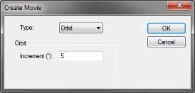
Orbit
In this mode, the contents of the scene are fixed and camera is rotated 360o. A frame of video is captured for the noted interval between frames.
Figure 11-24: Create Movie: Orbit
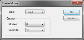
Timed
In this mode, the user’s action are recorded for a fixed amount of time.
Figure 11-25: Create Movie: Timed
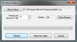
IES Movie Maker
Figure 11-26: IES Movie Maker
1. Movie Name: Click on this button to change the location where the file is saved as well as name of the file
2. Frame per second: This sets the frame rate
3. Extra Frames: You can add extra frames at the beginning of the file as a title card. This has to be a .BMP file
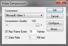
4. Settings: This contains options to change the various video compression techniques available for creating the videos.
Figure 11-27: Video Compression
5. Make the video: Save the video.