Chilled Water Loops, Pre-Cooling, Heat Rejection, and Chiller Sequencing
The chilled water loop tool provides access to selection, editing, and adding or removing named chilled water loops. Each individual chilled-water loop dialog then provides inputs for the following:
-
primary and secondary chilled water loops and option to use just one of these
-
pre-cooling devices such as integrated waterside economizers
-
chillers and other similar cooling sources (adding, sequencing, and editing of cooling equipment on the primary chilled-water loop)
-
heat-rejection loop (for water-cooled chillers) with cooling tower and options for waterside economizer and condenser heat recovery
A chilled water loop is associated with a chiller set comprising any number of chillers, which can include any combination of three different types:
-
electric water-cooled chiller (uses editable pre-defined curves and other standard inputs)
-
electric air-cooled chiller (uses editable pre-defined curves and other standard inputs)
-
part-load-curve chiller (flexible generic inputs; can represent any device used to cool water via a matrix of load-dependent data for COP and associated usage of pumps, heat-rejection fans, etc., with the option of adding COP values for up to four outdoor DBT or WBT conditions)
-
Each chiller or similar piece of water cooling equipment is defined in the context of a chilled water loop. Thus no chiller is permitted to serve more than one primary chilled water loop. Chillers can be duplicated using the Copy button within a chiller set and an “Import” facility is provided for copying a defined chiller from one chilled-water loop to another.
Heat rejection for water-cooled chillers is through an associated condenser water loop, for which an integrated waterside economizer is also available. Air-cooled chillers use only the design temperatures (DBT and WBT) for heat rejection. Heat rejection for the generic part-load-curve “chiller” type is described by the user via any combination of COP values, pump power, and fan power (all or any of which can be included in a composite COP) in the dialog for that type of equipment.
Cooling coils and chilled ceilings are assigned a chilled water loop rather than a chiller. The chilled water loop configuration can be either primary-only or primary-plus-secondary.
During simulation, chillers within a chiller set are switched in according to a user-specified sequence. During autosizing, sequenced chillers and the associated heat rejection plant and water flow rates are sized on the basis of user-specified percentages of the peak design load. Whether chillers are autosized or manually sized, the sizing of heat rejection equipment on the condenser water loop is always tied to the set cooling capacity of the chiller(s) that will operate maximum sequence load range. When electric-water-cooled chillers are included, and thus there is an associated cooling tower or fluid cooler, the chiller set may operate in waterside economizer mode (integrated or non-integrated modes are offered).
Chilled water loops are accessed through the toolbar button shown below.

Toolbar button for Chilled water loops.
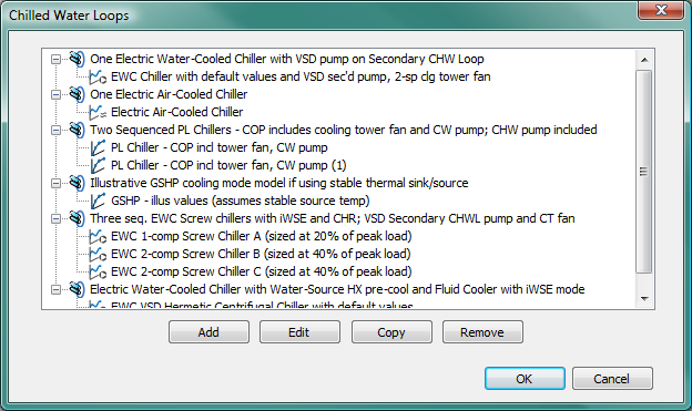
Clicking this toolbar button opens up the ‘Chilled water loops’ dialog (shown in Figure 2-17), which manages a set of chilled water loops. A chilled water loop may be added, edited, removed or copied through the corresponding buttons in this dialog. Double clicking on an existing chilled water loop (or clicking the ‘Edit’ button after selection of an existing chilled water loop) opens up the ‘Chilled water loop’ dialog (shown in Figure 3-63 ), where chilled water loop parameters may be edited.
The ‘Chilled water loop’ dialog currently has four tabs:
-
Chilled water loop tab: This tab manages the properties of the chilled water loop.
-
Pre-cooling tab: This tab manages pre-cooling devices to provide cooling on the chilled water loop (primary or secondary loop return) prior to the chiller set.
-
Chiller set tab: This tab manages a list of chillers (a chiller set), which may be edited with chiller dialogs (see section 2.5, 2.6 and 2.7). Chiller sequencing ranks under variable part load ranges are also defined in this tab, together with chiller autosizing capacity weightings.
-
Heat rejection tab: This tab manages information used for heat rejection. An optional condenser water loop for use by electric water-cooled chillers and (optionally) a waterside economizer can be defined in this tab.
Condenser water loop modeling
An optional condenser water loop is associated with each primary chilled water loop. This includes a cooling tower or fluid cooler model and is required only when the chiller set includes an electric water-cooled chiller (similarly, if a condenser water loop has been defined for a chilled water loop, at least one electric water-cooled chiller must also be defined for the same chilled water loop). An integrated waterside economizer is also available for condenser water loop systems.
Electric water-cooled chillers belonging to the same chiller set share a common condenser water loop and cooling tower or fluid cooler. The cooling tower model used is the same as that used for the Dedicated Water Side Economizer model, which is based on the Merkel theory. A condenser water pump is assumed to be included downstream of the cooling tower or fluid cooler.
When design condenser water flow rate differs from the rated condenser water flow rate, an adjustment is made to the entering condenser water temperature used by the program to solve for the chiller performance in the iteration process. The adjustment is made based on the following principle:
-
The effective entering condenser water temperature should be equal to the value that, for the given rate of heat rejection, would produce the same condenser water leaving temperature as a chiller operating with the rated condenser water flow rate.
The condenser water pump is assumed to operate in line with the electric water-cooled chiller(s) it serves and the optional waterside economizer operation mode of the condenser water loop. The condenser water flow rate is assumed to be constant at the design value when any electric water-cooled chiller on the loop is active and/or the condenser water loop is operating in waterside economizer mode. Condenser water pump power is the product of the flow rate and the rated specific pump power for the condenser water pump.
Chilled water loop configurations and pump modeling
There are two options for the Chilled water loop configuration:
-
Primary-only: Flow is maintained by a primary chilled water pump that can be either a variable-speed pump (i.e., using a variable-speed drive) or constant-speed pump riding the pump curve.
-
Primary-Secondary: Flow is maintained by a combination of primary and secondary pumps. The primary pump is assumed to have constant flow when it is on. The secondary pump can be either a variable-speed pump with VSD or a constant-speed pump riding the pump curve.
For both Chilled water loop configurations, when there is only a single chiller operating on the loop (i.e., without any pre-cooling devices or any waterside economizer or other chillers operating), the pump or pumps is/are assumed to operate only when the chiller is operating . In all other cases (i.e., when there are pre-cooling devices or waterside economizer or multiple chillers operating during the current simulation time step), the pump operation will be independent of the chiller on/off cycling status.
If a pump has variable flow rates (the primary pump in the Primary-only configuration or the secondary pump in the Primary-Secondary configuration), it will be subject to cycling on/off below the minimum flow rate permitted.
If the pump has a constant flow when it is on (the primary pump in the Primary-Secondary configuration ), this constant flow is multiplied by its specific pump power to determine the pump power. If the pump has variable flow (the primary pump in the Primary-only configuration, or the secondary pump in the Primary-Secondary configuration), i ts design pump power is calculated as the specific pump power multiplied by the design chilled water flow rate. The design pump power is then modified by the pump power curve to calculate the operating pump power at each simulation time step.
The variable flow featured in the pump power curve is calculated as the sum of required flows for all components served by the chilled water loop (cooling coils, chilled ceilings, etc.), subject to the minimum flow permitted for the pump. Required chilled water flow rates for simple cooling coils vary in proportion to their cooling loads, assuming a constant operating delta-T across the coils . The same is true for the r equired chilled water flow rates for chilled ceilings, except when chilled water loop supply temperature is specified to be used in the chilled ceiling control, in which case the r equired chilled water flow rates for chilled ceilings is calculated based on the detailed chilled ceiling heat transfer model with the chilled ceiling entering water temperature being equal to the chilled water loop supply temperature. Chilled water flow rates for advanced cooling coils are determined by the detailed heat transfer calculation of the advanced cooling coil model.
Chilled water and condenser water pump heat gains are modeled according to editable pump motor efficiency factors. Distribution losses from pipe work are considered as a user-specified percentage of the chilled water loop load.
Heat recovery
Heat rejected from a chilled water loop can be a heat recovery source either as collected directly from a part-load chiller model or via the condenser water loop serving one or more electric water-cooled chillers.
There are two options for modeling heat recovery:
-
Percentage of heat rejection : This is essentially the old heat recovery model provided in pre-v6.5 versions. It models the heat recovery as a simple percentage of the source heat rejection, with optional constant-COP water-source heat pump for upgrading the transferred heat. The fixed percentage represents simple heat-exchanger effectiveness. The temperature for the recovered heat can be upgraded with an electric water-to-water or water-source heat pump (WSHP). This would be used for adding recovered heat to hot water loops with higher temperatures—i.e., hotter than the condenser loop, in contrast to low-temperature hot-water heating systems for hydronic radiant floors, DHW pre-heat, or similar. Therefore, when serving space-heating loads, such as airside heating coils and baseboard heaters that require higher temperatures than normally available via a heat exchanger on the condenser water loop, this simple WSHP option can be used to account for energy used to upgrade the temperature (e.g., from 90°F to 140°F). The Percentage of heat rejection model can be used regardless of whether there is an explicit modeling of the loop water temperatures on the heat recovery source and recipient sides.
-
Explicit heat transfer : This more detailed heat recovery model was added in v6.5. It transfers heat between the source and recipient loops using an explicit water-to-water heat exchanger model with effectiveness that is continuously modulated for off-design temperature differences across the heat exchanger. In the explicit heat transfer model, the water-to-water heat pump (WWHP) used to upgrade the heat recovery is enhanced by the inclusion of a COP that varies according to thermal lift between the heat recovery source loop and recipient loops during the simulation: Linear interpolation is applied to 1/COP to modulate between two heat pump COP values corresponding to two operational data points specified by the user (low thermal lift and high thermal lift). The Explicit heat transfer model can be used only with explicit modeling of the loop water temperatures on the heat recovery source and recipient sides—i.e., with the condenser water loop model as source and hot water loop or heat transfer loop model as the recipient.
Capacity for the Heat Recovery WWHP is now limited to a user-specified percentage of the heat recovery source capacity, whereas in pre-v6.5 versions WWHP capacity was a percentage of the instantaneous load on the source. This revised limit has been introduced in both of the WWHP models described above in order to provide a more realistic basis for the capacity. This avoids recovering more heat with the WWHP than would be possible (or desirable) in practice. For example, without this constraint the WWHP could entirely displace the boilers on a HWL, which might not be what the user intends or expects.
Heat recovery sources and recipients
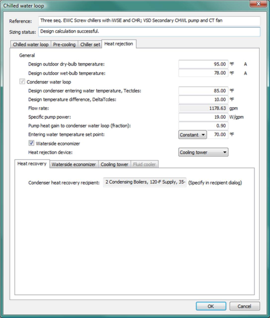
All heat recovery data are now displayed, edited, and stored on the recipient side (see Figure 3-16 and Figure 3-17 in the section on Hot water loop modeling). The heat recovery recipient is displayed on the source side (Heat recovery sub-tab within the Heat Rejection tab of the Chilled water loop dialog and within the Part-load curve chiller model dialog) for user’s information only. Each heat recovery source can be linked to only one heat recovery recipient, and this is done from the recipient side.
Heat recovery sources can be either a part-load-curve “chiller” model (which may represent something other than a water-cooled chiller) or a condenser water loop serving one or more electric water-cooled chillers. Future versions will expand on the range of possible sources, for example, allowing the heat-transfer loop to be selected as a source. Heat recovery recipients can be a generic heat source, a hot water loop, or a heat transfer loop.
When the Percentage of heat rejection model is used, there can be multiple heat recovery sources linked to one recipient. This is among the reasons that the sources are now specified in the recipient dialog. Source types can be any combination of condenser water loops and/or part-load curve chiller models. Each heat recovery source can be linked to just one heat recipient.
When the Explicit heat transfer model is used, there can be only one heat recovery source linked to a given recipient loop. The recipient can be a hot water loop or heat transfer loop and the source type is limited to condenser water loops—i.e., there must be an explicit model of the loop temperatures and flow rates on both sides of the heat exchanger or heat pump.
Figure 3 - 63 : Chilled water loops dialog (shown with default and illustrative loops included with the pre-defined systems)
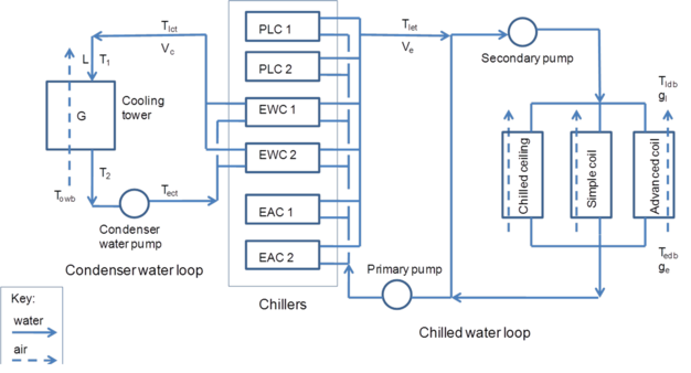
Figure 3 - 64 : Chilled water loop configuration drawn with a chiller set that includes all three types of chiller models (part-load-curve; electric water-cooled; electric air-cooled): only the electric water-cooled type is couple to the condenser water loop and cooling tower model. See 2.10.11 Primary Circuit Chilled Water Specific Pump Power for modeling systems having only a primary chilled water loop—no secondary loop.
Chilled water loop dialog
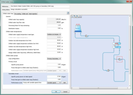
Figure 3 - 65 : Chilled water loop editing dialog (shown with the Chilled water loop tab active)
Figure 3 - 66 : Chilled water loop tab in the Chilled water loop dialog (shown with inputs for an illustrative loop configuration and settings as included with the pre-defined systems)
Reference name for Chilled Water Loop
Enter a description of the component. It is for your use when selecting, organizing, and referencing any component or controllers within other component and controller dialogs and in the component browser tree. These references can be valuable in organizing and navigating the system and when the system model is later re-used on another project or passed on to another modeler. Reference names should thus be informative with respect to differentiating similar equipment, components, and controllers.
Chilled Water Loop tab
The Chiller water loop tab facilitates the definition of the chilled water temperatures and chilled water pumps, together with the distribution losses and oversizing factor for the chilled water loop.
Chilled water loop capacity
This is a derived parameter calculated from the user-specified supply water temperature and the flow rate required to deliver the cooling capacity of attached chillers at the Design condition, including the minimum specified supply water temperature.
Chilled water loop flow rate
This is the derived flow rate required to deliver the Design cooling capacity of attached chillers at the Design (minimum) supply water temperature.
Oversizing Factor
This is the oversizing factor that will be used in the autosizing of this component. During autosizing the capacity will be set to the peak load multiplied by the oversizing factor.
Distribution Losses
Enter the chilled water loop distribution losses—i.e., the loss due to distribution of cooling from the cooling plant equipment to point of use—as a percentage of cooling demand. The loss entered here is not recouped in the building.
|
Warning Limits (%)
|
0.0 to 20.0
|
|
Error Limits (%)
|
0.0 to 75.0
|
Chilled Water Supply Temperature Reset Type
Select the chilled water supply temperature reset type. Currently two options are provided: No reset or Outdoor air temperature reset. When Outdoor air temperature reset type is selected, which is the default, you also need to specify four more reset parameters:
· Outdoor dry-bulb temperature low limit
· Chilled water supply temperature at or below low limit
· Outdoor dry-bulb temperature high limit
· Chilled water supply temperature at or above high limit
When No reset is selected, you need only specify the constant design chilled water supply temperature.
Chilled Water Supply Temperature
Enter the design chilled water supply temperature (leaving evaporator water temperature) if the chilled water supply temperature reset type is selected as No reset. When Chilled water supply temperature reset type is selected as Outdoor air temperature reset, this field becomes inactive.
Outdoor Dry-bulb Temperature Low Limit
When chilled water supply temperature reset type is selected as Outdoor air temperature reset, enter the outdoor dry-bulb temperature low limit to be used by the reset.
Chilled Water Supply Temperature at or below Low Limit
When chilled water supply temperature reset type is selected as Outdoor air temperature reset, enter the chilled water supply temperature to be used by the reset at or below the outdoor dry-bulb temperature low limit.
Outdoor Dry-bulb Temperature High Limit
When chilled water supply temperature reset type is selected as Outdoor air temperature reset, enter the outdoor dry-bulb temperature high limit to be used by the reset.
Chilled Water Supply Temperature at or above High Limit
When chilled water supply temperature reset type is selected as Outdoor air temperature reset, enter the chilled water supply temperature to be used by the reset at or above the outdoor dry-bulb temperature high limit.
Design Chilled Water Loop Temperature Difference (∆Tedes)
Enter the design chilled water loop temperature difference (∆T edes )—i.e., the difference between the design chilled water supply and return temperatures.
Loop Configuration
Select the loop configuration. Two options are offered: Primary-only and Primary-Secondary.
When loop configuration is set to Primary only, there is just one chilled water pump (fixed or variable-speed) and Primary return is the only option provided for the location of pre-cooling devices and waterside economizer (this is in the Location of pre-cooling loop drop-down menu on Pre-cooling tab and in the Location of waterside economizer drop-down menu on the Waterside economizer sub-tab in the Heat rejection tab).
When loop configuration is set to Primary-Secondary, the primary pump is a fixed-speed pump, a separate pump (fixed or variable-speed) is added for the secondary loop, and the available options for the location of pre-cooling devices and waterside economizer can be either Primary return or Secondary return, with the assumption that heat exchanger for waterside economizer operation using the condenser water loop will always be downstream of any dedicated pre-cooling device.
Variable flow vs. variable speed and pipe configuration vs. pump location: The secondary pump is always modeled with variable flow characteristics, either using a variable-speed pump or using a constant speed pump riding the pump curve (i.e. the flow rate on the secondary loop can be varied by valves on the loop even when the pump motor is operating at a constant speed). As a function of the chiller model, the primary pump in this case is modeled on a constant flow basis. The secondary variable flow pump can still be a constant speed pump or a variable speed pump, depending on the performance curve (constant speed or variable speed) selected for the secondary pump.
Regardless of the pump configuration, the loop pipe system is the same. So for the primary only configuration, the pipe flow through the primary pump is actually the secondary flow. i.e., the primary pump is located on the secondary pipe, and there is no pump on the primary pipe. The reason for this is that most users wish to model primary-only systems with variable flow (placing the primary pump in the primary pipe for the primary-only configuration would cause the primary pump to be modeled on a constant flow basis). While for the primary-secondary configuration, the primary pump is located on the primary pipe, and the secondary pump is located on the secondary pipe.
The loop configuration is always used to refer to the presence of pumps.
• For primary-secondary: this means both primary pump and secondary pump are present and are modeled in Apache.
• For primary only: this means only primary pump is present and is modeled in Apache. However, the primary pump in the primary-only configuration is actually located on the secondary loop pipe and is modeled in the same way as the secondary pump of the primary-secondary configuration, i.e., it is modeled as a variable ‘flow’ pump located on the secondary loop pipe. It is called ‘Primary only’ because it is the only pump present on the loop.
Note regarding pump configurations in older HVAC system files (prior to VE 2012 Feature Pack 2):
When loading an older network with a secondary-only variable flow pump configuration that was used to model a variable-flow primary-only configuration wherein both the primary and secondary pumps are technically still present on the loop, but the specific pump power of the primary pump in this configuration is set to zero so that all primary pump power, pump heat gain, pump temperature rise etc. will be calculated to be zero (leaving the secondary pump with variable flow to be seen as the only active pump and therefore the “primary” pump), this will be represented in exactly as it was in older versions of ApacheHVAC. The only difference is the Chilled water pumps section in Chilled water loop tab of the Chilled water loop dialog will now have a new parameter: Loop configuration, which will have two options: Primary-Secondary and Primary only. All old networks with chilled water loops will have this new parameter set to Primary-Secondary, as this was the only option available for chilled water loops prior to VE 2012 Feature Pack 2. (Loop configuration was not explicitly displayed on the old interface).
Primary Circuit Chilled Water Specific Pump Power at Rated Speed
Enter the primary circuit chilled water specific pump power at rated speed, expressed in W/(l/s) in SI units (or W/gpm in IP units).
When loop configuration is set to Primary-only:
Primary circuit chilled water pump power is calculated on the basis of variable flow, subject to the constraint that the pump will start cycling below the minimum flow rate permitted by the Minimum V (min volumetric flow rate fraction) parameter set in the pump curve editing dialog. Design pump power is the product of specific pump power multiplied by the design chilled water flow rate. Then operating pump power is then based on the design pump power modified by the pump power curve. The default value for the specific pump power for primary-only configurations is the total chilled water specific pump power (22 W/gpm) specified in ASHRAE standard 90.1 G3.1.3.10.
The variable flow featured in the pump power curve is calculated as the sum of required flows for all components (cooling coils, chilled ceilings, etc.) served by the chilled water loop, subject to the minimum flow permitted for the pump. Required chilled water flow rates for simple cooling coils vary in proportion to their cooling loads assuming a constant operating delta-T across the cooling coils. The same is true for the r equired chilled water flow rates for chilled ceilings, except when chilled water loop supply temperature is specified to be used in the chilled ceiling control, in which case the r equired chilled water flow rate for chilled ceilings is calculated based on the detailed chilled ceiling heat transfer model with the chilled ceiling entering water temperature being equal to the chilled water loop supply temperature. Chilled water flow rates for advanced cooling coils are determined by the detailed heat transfer calculation of the advanced cooling coil model.
When loop configuration is set to Primary-Secondary:
Primary circuit chilled water pump power will be calculated on the basis of constant flow (when the chiller operates). The model will be based on a specific pump power parameter, with a default value of 4.4 W/gpm. The default value is based on the total chilled water specific pump power (22 W/gpm) as specified in ASHRAE standard 90.1 G3.1.3.10, assuming a 20:80 split between the primary and secondary circuits. The basis for this default split is described under Secondary Circuit Chilled Water Specific Pump Power at Rated Speed, below.
The primary circuit chilled water loop flow rate is calculated from the design cooling capacity (Qdes) and the design chilled water temperature change (∆Tedes) of the chilled water loop.
Primary Circuit Chilled Water Pump Heat Gain to Chilled Water Loop (fraction)
Enter the primary circuit chilled water pump heat gain to chilled water loop, which is the fraction of the motor power that ends up in the Chilled water. Its value is multiplied by the primary circuit chilled water pump power to get the primary circuit chilled water pump heat gain, which is added to the cooling load of the chilled water loop.
Primary Circuit Chilled Water Pump Performance Curve, fPv(v)
This field is active only when Loop configuration is set to Primary-only.
This line of the dialog displays the short description and curve name for the currently selected primary loop chilled water pump power curve. Use the dropdown list to select the appropriate curve from the system database. Use the Edit button to edit the curve parameters if needed. The Edit button opens a dialog displaying the formula and parameters of the curve. Curve coefficients and applicable ranges of the independent variables are editable.
When editing curve parameters, it is important to understand the meaning of the curve and its usage in the model algorithm. It is also important that the edited curve has reasonable applicable ranges for the independent variables. A performance curve is valid only within its applicable ranges. If the independent variables are out of the set applicable ranges, the variable limits (maximum or minimum) specified in the input will be applied.
The primary circuit chilled water pump power curve f Pv (v) is a cubic function of
v = V/V e
where
V = pump volumetric flow rate.
V e = design pump volumetric flow rate.
And:
f Pv (v) = (C 0 + C 1 v + C 2 v 2 + C 3 v 3 ) / C norm
where
C 0 , C 1 , C 2 and C 3 are the curve coefficients
C norm is adjusted (by the program) to make f Pv (1) = 1
The primary circuit chilled water pump power curve is evaluated for each iteration of the chilled water loop, for each time step during the simulation. The curve value is multiplied by the design primary chilled water pump power to get the operating primary pump power of the current time step, for the current fraction of pump volumetric flow rate. The curve should have a value of 1.0 when the operating pump volumetric flow rate is equal to the rated pump volumetric flow rate (v = 1.0).
Figure 3 - 67 : Edit dialog for the primary circuit chilled water pump power curve (values for constant-speed pump are shown).
Secondary Circuit Chilled Water Specific Pump Power at Rated Speed
This field is active only when Loop configuration is set to Primary-Secondary.
Enter the secondary circuit chilled water specific pump power at rated speed, expressed in W/(l/s) in SI units (or W/gpm in IP units). The default value (17.6 W/gpm) is based on the total chilled water specific pump power (22 W/gpm) as specified in ASHRAE 90.1 G3.1.3.10 and assuming a 20:80 split between the primary and secondary circuits. The default 20:80 split between primary and secondary is based upon typical pump head values of 15 feet of head for the primary loop and 60 feet of head for the secondary loop. Thus the default specific pump power values are 4.4 W/gpm or 69.7414 W/(l/s) for the primary loop, and 17.6 W/gpm or 278.9657 W/(l/s) for the secondary loop. However, while this default may be appropriate to 90.1 PRM Baseline models, it is otherwise just a typical starting point and should be adjusted to match the actual relative pump head values.
Secondary circuit chilled water pump power at each simulation time step is calculated on the basis of variable flow. Required chilled water flow rates for simple cooling coils and chilled ceilings vary in proportion to their cooling loads, assuming a constant operating delta-T across the cooling coils. The same is true for the chilled water flow rates r equired by chilled ceilings, except when chilled water loop supply temperature is specified to be used in the chilled ceiling control, in which case the r equired chilled water flow rate for chilled ceilings is calculated based on the detailed chilled ceiling heat transfer model with the chilled ceiling entering water temperature being equal to the chilled water loop supply temperature. Chilled water flow rates for advanced cooling coils are determined by the detailed heat transfer calculation of the advanced cooling coil model. Required chilled water flow rates from all cooling coils and chilled ceilings served by a chilled water loop are summed to get the required secondary circuit chilled water flow rate, subject to the minimum flow rate permitted for the pump (Minimum V in the pump curve edit dialog).
The design secondary circuit chilled water loop flow rate is assumed equal to the design primary circuit chilled water loop flow rate, which is calculated from the design cooling capacity (Q des ) and the design chilled water temperature change ∆T edes .
The design secondary chilled water pump power is calculated as the secondary specific pump power multiplied by the design secondary chilled water flow rate. It is then modified by the secondary circuit pump power curve to get the operating secondary pump power.
Secondary Circuit Chilled Water Pump Heat Gain to Chilled Water Loop (fraction)
This field is active only when Loop configuration is set to Primary-Secondary.
Enter the secondary circuit chilled water pump heat gain to chilled water loop, which is the fraction of the motor power that ends up in the Chilled water. Its value is multiplied by the secondary circuit chilled water pump power to get the secondary circuit chilled water pump heat gain, which is added to the cooling load of the chilled water loop.
Secondary Circuit Chilled Water Pump Power Curve, fPv(v)
This field is active only when Loop configuration is set to Primary-Secondary.
This line of the dialog displays the short description and curve name for the currently selected secondary loop chilled water pump power curve. Use the dropdown list to select the appropriate curve from the system database. Use the Edit button to edit the curve parameters if needed. The Edit button opens a dialog displaying the formula and parameters of the curve. Curve coefficients and applicable ranges of the independent variables are editable.
When editing curve parameters, it is important to understand the meaning of the curve and its usage in the model algorithm. It is also important that the edited curve has reasonable applicable ranges for the independent variables. A performance curve is valid only within its applicable ranges. If the independent variables are out of the set applicable ranges, the variable limits (maximum or minimum) specified in the input will be applied.
The secondary circuit chilled water pump power curve f Pv (v) is a cubic function of
v = V/V e
where
V = pump volumetric flow rate.
V e = design pump volumetric flow rate.
And:
f Pv (v) = (C 0 + C 1 v + C 2 v 2 + C 3 v 3 ) / C norm
where
C 0 , C 1 , C 2 and C 3 are the curve coefficients
C norm is adjusted (by the program) to make f Pv (1) = 1
The secondary circuit chilled water pump power curve is evaluated for each iteration of the chilled water loop, for each time step during the simulation. The design secondary chilled water pump power is multiplied by the curve value to get the operating secondary pump power of the current time step, for the current fraction of pump volumetric flow rate. The curve should have a value of 1.0 when the operating pump volumetric flow rate equals rated pump volumetric flow rate (v = 1.0).
Example:
The standard curve for a variable-speed pump at 60% of the design flow rate will return a value of 0.216. Assume for this example that the design flow rate is 100 gpm, thus 60% would be 60 gpm. If the specific pump power at the design flow rate were 15 W/gpm, this would equate to 1,500 W at design flow. Finally, the 1,500 W pump power at the design flow would be multiplied by 0.216 to yield 324 W pump power at 60% of the design flow rate. If the input for “Minimum v” in the pump performance curve Edit dialog were set to 0.600 or 60% minimum pump operating volume, this would cause the secondary pump power to remain at 324 W whenever the pump operates at or below the 60% minimum setting for the volumetric flow rate.
As noted in previous sections, the secondary circuit chilled water pump is assumed to operate in line with the chiller(s)—i.e., the pump is on whenever one or more chiller is active; however, the pump will cycle whenever the required flow rate is at or below the set minimum flow rate for the pump (Minimum v in the performance curve Edit dialog), regardless of whether or not the first chiller in the sequence has reached the set minimum load fraction for continuous chiller operation. When the pump is on, the pump power is calculated as the design pump power multiplied by the pump curve value for the minimum v point on the curve. When cycled off, the pump power is zero.
When the pump operates in line with the chiller, it will cycle on/off with the chiller as well—i.e., when the loop cooling load is below the set minimum load fraction for continuous chiller operation. The chiller cycling ratio associated with the load fraction for at each simulation time step will thus be used in the pump power calculation when the pump is cycling on and off as a result of the chiller doing so. If the require water flow rate is also at or below minimum for the pump, the pump power calculated as the design pump power multiplied by the pump curve value at the minimum v will be multiplied by both the chiller running fraction and the pump running fraction.
Figure 3 - 68 : Edit dialog for the secondary circuit chilled water pump power curve (values for constant-speed pump are shown)
Pre-cooling tab
The Pre-cooling tab ( Figure 3-69 ) provides for the specification of pre-cooling devices on the chilled water loop. These devices can either pre-cool the chilled water return before it re-enters the chiller set or, when there is sufficient pre-cooling capacity with respect to cooling load, provide all necessary return water cooling. Pre-cooling devices can be located either on the return of either the Primary or Secondary chilled water loop.
Figure 3 - 69 : Pre-cooling tab on Chilled water loop dialog (shown with inputs for an illustrative integrated water-source heat exchanger as autosizable pre-cooling device on the secondary CHWL return)
Design outdoor dry-bulb temperature
Enter the design outdoor dry-bulb temperature for the pre-cooling device(s).
Design outdoor wet-bulb temperature
Enter the design outdoor wet-bulb temperature for the pre-cooling device(s). Design outdoor wet-bulb temperature has to be lower than design outdoor dry-bulb temperature.
Location of pre-cooling loop
Select the location of the pre-cooling device.
Pre-cooling devices can be placed on the return of either the chilled water loop primary or secondary circuits. If placed on the primary loop, the device is placed downstream of the primary pump. If placed on the secondary loop, the device is located immediately upstream of the primary-secondary common pipe junction. In the current implementation, all pre-cooling devices must use the same location.
Pre-cooling capacity
The capacity of pre-cooling devices on the chilled water loop can be sized as either a percentage of total loop capacity or by an explicit capacity value. When the % of CHWL capacity box is checked, the Capacity value will be derived from the entered percentage and the chilled water loop capacity. In this instance, the pre-cooling capacity may be autosized. When the box is unchecked, the capacity must be entered explicitly. Pre-cooling devices cannot have a capacity greater than the chilled water loop capacity (% of CHWL capacity cannot exceed 100%).
Heat rejection devices
Pre-cooling devices on the chilled water loop include a water source heat exchanger, a cooling tower with heat exchanger, and a fluid cooler. Checking the box for Water source heat exchanger will activate the water source heat exchanger sub-tab, allowing the user to edit the parameters of the heat exchanger. Checking the box for Ambient device enables a pull-down menu where users can selected either a cooling tower with heat exchanger or fluid cooler as a pre-cooling device. Depending upon the ambient device selected, the appropriate sub-tab will be active for editing.
The water source heat exchanger can be used in series for pre-cooling with either the cooling tower with heat exchanger or fluid cooler.
Water source heat exchanger Cooling capacity
The capacity of the water source heat exchanger can be sized as either a percentage of total pre-cooling device capacity or by an explicit capacity value. When the % of PC capacity box is checked, the Capacity value will be derived from the entered percentage and the pre-cooling capacity. When the box is unchecked, the capacity must be entered explicitly. The water source heat exchanger cannot have a capacity greater than the pre-cooling capacity (% of PC capacity cannot exceed 100%).
Water source heat exchanger Source water temperature
Two options are available for the water-source heat exchanger source water temperature: Constant or Profiled.
When Source water temperature is selected as Constant (which is the default), the Source-side entering temperature in the Design parameters section is a dynamic copy of the Constant source water temperature specified in the Source water section. In this case, the Design source-side entering temperature is derived parameter and hence not editable.
When Profiled is selected for Source water temperature, select the absolute profile to be applied to the water-source heat exchanger source water temperature, which is defined through the APPro facility (the Profiles Database).
When Source water temperature is selected as Profiled, the Source-side entering temperature in the Design parameters section is an input parameter and hence editable. In this case, as it is hard to automatically ensure the design source-side entering temperature value falls within the range set by the source water temperature profile, it will be the user’s responsibility to ensure the design source-side entering temperature is available from the temperature profile defined for the source water.
Water source heat exchanger Source water specific pump power
Enter the specific pump power for the water-source heat exchanger source water pump, expressed in W/(l/s) in SI units (or W/gpm in IP units).
Water source heat exchanger Source water pump meter
Select the appropriate energy meter for the source water pump. If it is desired to sub-meter the source water pumping energy separate from the other Electricity use in the model, or separate from the other pumping energy, users may create an Electricity meter in Apache that will, after creation, be selectable here.
Water source heat exchanger Load-side Design parameters
Load-side flow rate for the water-source heat exchanger is always a dynamic copy of the Loop flow rate from the Chilled water loop tab. It is automatically derived by the software and does not need to be specified.
Load-side delta T for the water-source heat exchanger is the temperature difference between the heat exchanger load-side leaving temperature and load-side entering temperature. It is automatically derived by the software and does not need to be specified.
Load-side leaving temperature for the water-source heat exchanger is automatically derived by the software and does not need to be specified. It is the difference between the Source-side entering temperature and the Approach for the water source heat exchanger.
Water source heat exchanger Source-side entering temperature
When Source water temperature is selected as Constant (which is the default), the Source-side entering temperature in the Design parameters section is a dynamic copy of the Constant source water temperature specified in the Source water section. In this case, the Design source-side entering temperature is derived parameter and hence not editable.
When Source water temperature is selected as Profiled, the Source-side entering temperature in the Design parameters section is an input parameter and hence editable. In this case, as it is hard to automatically ensure the design source-side entering temperature value falls within the range set by the source water temperature profile, it will be the user’s responsibility to ensure the design source-side entering temperature is available from the temperature profile defined for the source water.
Water source heat exchanger Approach
Design approach of a water-to-water heat exchanger is defined as the absolute temperature difference between its load-side leaving temperature and source-side entering temperature.
Water source heat exchanger Heat exchanger effectiveness
Heat exchanger effectiveness is automatically derived by the software using other parameters specified for the water-source heat exchanger and does not need to be specified. Note that feasible heat exchanger effectiveness (ɛ) should be: 0.0 ≤ ɛ ≤ 1.0. When the heat exchanger design effectiveness derived using the specified heat exchanger parameters is out of the feasible range, the Sizing status at the top of the Chilled water loop dialog will report an error message in red text and a mouse-over tip over the out-of-range effectiveness (shown as red value in the field) will be given to adjust the heat exchanger parameters so that a feasible effectiveness can be derived.
Water source heat exchanger Source-side delta T
Source-side delta T for the water-source heat exchanger is the temperature difference between the heat exchanger source-side leaving temperature and source-side entering temperature.
Given the heat exchanger capacity, the calculation of the Source-side delta T and the Source-side flow rate (see below) is interchangeable. You can choose to either enter the Source-side delta T or the Source-side flow rate and the software will automatically derive the other. The “[” symbol besides the Source-side delta T and the Source-side flow rate fields indicates this interchangeable relation.
Water source heat exchanger Source-side flow rate
Given the heat exchanger capacity, the calculation of the Source-side delta T (see above) and the Source-side flow rate is interchangeable. You can choose to either enter the Source-side delta T or the Source-side flow rate and the software will automatically derive the other. The “[” symbol besides the Source-side delta T and the Source-side flow rate fields indicates this interchangeable relation.
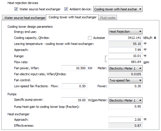
Figure 3 - 70 : Cooling tower with heat exchanger sub-tab of the Pre-cooling tab on Chilled water loop dialog
Cooling tower Energy end use
When used as a pre-cooling device, a cooling tower may serve either heat rejection or cooling purposes. Users should select the appropriate energy end use for the cooling tower in their application. Selection of this end use does not affect the performance of the cooling tower, only the reporting of energy results.
Cooling tower Cooling capacity, Qhrdes
This is the pre-cooling load on the cooling tower at design condition. The capacity of the cooling tower can be autosized or explicitly entered by the user. If the autosize check box is utilized, the cooling tower will size to make up the difference between the pre-cooling loop capacity and the water source heat exchanger cooling capacity (if also present on the pre-cooling loop).
Cooling tower with heat exchanger Leaving temperature
Leaving water temperature for the cooling tower with heat exchanger is the design outdoor dry-bulb temperature for the pre-cooling loop added to the heat exchanger approach. It is automatically derived by the software and does not need to be specified.
Cooling tower Approach
This is the difference between the cooling tower leaving water temperature and the outdoor dry-bulb temperature at the design condition.
Cooling tower Range
This is the difference between the cooling tower entering water temperature and the cooling tower leaving water temperature at the design condition.
Given the heat exchanger capacity, the calculation of the Range and the Flow rate (see below) is interchangeable. You can choose to either enter the Range or the Flow rate and the software will automatically derive the other. The “[” symbol besides the Range and the Flow rate fields indicates this interchangeable relation.
Cooling tower Flow rate
Given the cooling tower capacity, the calculation of the Range (see above) and the Flow rate is interchangeable. You can choose to either enter the Range or the Floe rate and the software will automatically derive the other. The “[” symbol besides the Range and the Flow rate fields indicates this interchangeable relation.
Cooling tower Fan power, Wfan
Enter the power consumption of the cooling tower fan when running at full speed.
Cooling tower Fan Meter
Select the appropriate energy meter for the cooling tower fan. If it is desired to sub-meter the fan energy separate from the other Electricity use in the model, or separate from the other heat rejection/cooling energy, users may create an Electricity meter in Apache that will, after creation, be selectable here.
Cooling tower Fan electric input ratio, Wfan/Qhrdes
This is the ratio between the design fan power consumption and the design heat rejection load of the cooling tower. It is automatically derived by the program using the provided cooling tower fan power and the derived cooling tower design heat rejection load, and does not need to be specified.
Cooling tower Fan control
Select the fan control type of the cooling tower. Three types of fan control are available
· One-speed fan
· Two-speed fan
· VSD fan
When Two-speed fan is selected, you also need to specify two more parameters (see below): Low-speed fan flow fraction and Low-speed fan power fraction.
Cooling tower Low-speed Fan Flow Fraction
Enter the fraction of the design flow that the cooling tower fan delivers when running at low speed. This parameter only needs to be specified when Fan control type is selected as Two-speed fan.
Cooling tower Low-speed Fan Power Fraction
Enter the power consumed by the cooling tower fan when running at low speed, expressed as a fraction of the cooling tower design fan power. This parameter needs only to be specified when Fan control type is selected as Two-speed fan. Generally, the low-speed power fraction will be a lesser value than the low-speed flow fraction. For example, if the low-speed flow fraction were 0.50, the low-speed power fraction would typically (depending on fan curves, motor performance, etc.) be on the order of 0.30.
Cooling tower Specific Pump Power
Enter the cooling tower water specific pump power at rated speed, expressed in W/(l/s) in SI units (or W/gpm in IP units).
Cooling tower water pump power will be calculated on the basis of constant flow (whenever the pre-cooling loop is engaged). The model will be based on a specific pump power parameter, with a default value of 19 W/gpm as specified in ASHRAE 90.1 G3.1.3.11.
Cooling tower Pump Meter
Select the appropriate energy meter for the cooling tower pump. If it is desired to sub-meter the pump energy separate from the other Electricity use in the model, or separate from the other heat rejection/cooling energy, users may create an Electricity meter in Apache that will, after creation, be selectable here.
Cooling tower Pump heat gain to cooling tower loop (fraction)
Enter the cooling tower water pump heat gain to the cooling tower water loop, which is the fraction of the pump motor power that ends up in the cooling tower water. Its value is multiplied by the cooling tower water pump power to get the cooling tower water pump heat gain, which is added to the pre-cooling load of the cooling tower. (Cooling tower water pump is assumed to be on the supply side of the cooling tower.)
Cooling tower with heat exchanger Heat exchanger Approach
Design approach of a water-to-water heat exchanger is defined as the absolute temperature difference between its load-side (pre-cooling loop) leaving temperature and source-side entering temperature (cooling tower leaving temperature).
Cooling tower with heat exchanger Heat exchanger Effectiveness
Heat exchanger effectiveness is automatically derived by the software using other parameters specified for the cooling tower heat exchanger and does not need to be specified. Note that feasible heat exchanger effectiveness (ɛ) should be: 0.0 ≤ ɛ ≤ 1.0. When the heat exchanger design effectiveness derived using the specified heat exchanger parameters is out of the feasible range, the Sizing status at the top of the Chilled water loop dialog will report an error message in red text and a mouse-over tip over the out-of-range effectiveness (shown as red value in the field) will be given to adjust the heat exchanger parameters so that a feasible effectiveness can be derived.
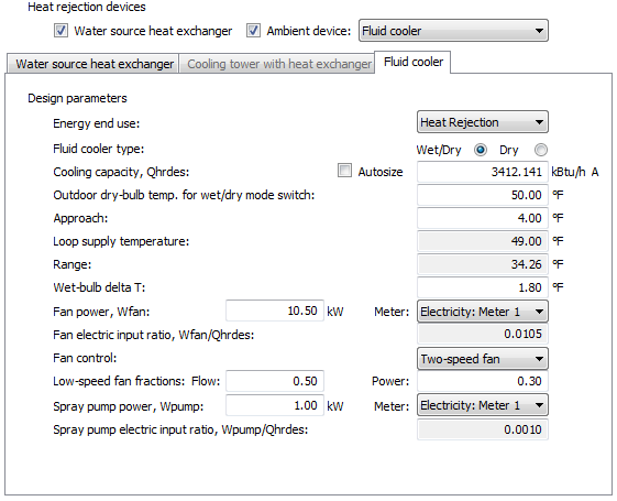
Figure 3 - 71 : Fluid cooler sub-tab of the Pre-cooling tab on Chilled water loop dialog
Fluid Cooler Energy End Use
When used as a pre-cooling device, a fluid cooler may serve either heat rejection or cooling purposes. Users should select the appropriate energy end use for the fluid cooler in their application. Selection of this end use does not affect the performance of the fluid cooler, only the reporting of energy results.
Fluid Cooler Type
There are two types of fluid coolers, categorized by the wetting conditions on the surface of the coil.
A dry fluid cooler is one where the coil is permanently dry—i.e., evaporative cooling is not included. This type of cooler tends to be used in areas where there are restrictions on the availability of water or where ambient conditions are particularly well suited to a dry cooler.
A wet/dry fluid cooler is one where the coil is sprayed with water to provide indirect evaporative cooling. To prevent freezing of water on the coil and/or to make the most of cool conditions, the spray pump can be switched off at low outdoor temperatures. Under these conditions the cooler operates with a dry coil.
This radio button group allows the type of fluid cooler to be selected.
Fluid Cooler Cooling Capacity, Qhrdes
This is the pre-cooling load on the fluid cooler at design condition. The capacity of the fluid cooler can be autosized or explicitly entered by the user. If the autosize check box is utilized, the fluid cooler will size to make up the difference between the pre-cooling loop capacity and the water source heat exchanger cooling capacity (if also present on the pre-cooling loop).
Fluid Cooler Outdoor Dry-Bulb Temperature for Wet/Dry Mode Switch
When a wet/dry fluid cooler has been selected this value is used to define the temperature at which the mode of the fluid cooler changes. When the outdoor dry-bulb temperature falls below the value specified, the fluid cooler will run in dry mode, the spray pump is turned off and the coil will be dry. When the outdoor dry-bulb temperature is above the value set, the spray pump will be in operation and the coil will be wet (evaporatively cooled).
Fluid Cooler Approach
When the fluid cooler is operating in wet/dry mode, this is the difference between the fluid cooler leaving water temperature and the outdoor wet-bulb temperature at the design condition. In dry mode, this value is the difference between the leaving water temperature and the outdoor dry-bulb temperature at the design condition.
Fluid Cooler Loop Supply Temperature
The fluid cooler loop supply temperature is derived from the fluid cooler approach (see above) and the design outdoor temperatures. For a wet/dry fluid cooler, the Approach is added to the Design outdoor wet-bulb temperature. For a dry fluid cooler, the Approach is added to the Design outdoor dry-bulb temperature.
Fluid Cooler Range
This is the difference between the fluid cooler entering water temperature and the fluid cooler leaving water temperature at the design condition. The design range of the fluid cooler is automatically derived by the program using the provided pre-cooling loop design data and pump data. It does not need to be specified.
Fluid Cooler ∆T
For the fluid cooler in wet/dry mode, this is the difference between the fluid cooler exiting wet-bulb air temperature and entering wet-bulb air temperature. In dry mode this is the difference between the exiting dry-bulb air temperature and the entering dry-bulb air temperature.
Fluid Cooler Fan Power, Wfan
The power consumption of the fluid cooler fan when running at full speed.
Fluid Cooler Fan Meter
Select the appropriate energy meter for the fluid cooler fan. If it is desired to sub-meter the fan energy separate from the other Electricity use in the model, or separate from the other heat rejection/cooling energy, users may create an Electricity meter in Apache that will, after creation, be selectable here.
Fluid Cooler Fan Electric Input Ratio, Wfan/Qhrdes
This is the ratio between the design fan power consumption and the design heat rejection load of the fluid cooler. It is automatically derived by the program using the provided fluid cooler fan power and the derived fluid cooler design heat rejection load. It does not need to be specified.
Fluid Cooler Fan control
Select the fan control type of the cooling tower. Three types of fan control are available
· One-speed fan
· Two-speed fan
· VSD fan
When Two-speed fan is selected, you also need to specify two more parameters (see below): Low-speed fan flow fraction and Low-speed fan power fraction.
Fluid Cooler Low-speed Fan Flow Fraction
Enter the fraction of the design flow that the fluid cooler fan delivers when running at low speed. This parameter only needs to be specified when Fan control type is selected as Two-speed fan.
Fluid Cooler Low-speed Fan Power Fraction
Enter the power consumed by the fluid cooler fan when running at low speed, expressed as a fraction of the fluid cooler design fan power. This parameter needs only to be specified when Fan control type is selected as Two-speed fan. Generally, the low-speed power fraction will be a lesser value than the low-speed flow fraction. For example, if the low-speed flow fraction were 0.50, the low-speed power fraction would typically (depending on fan curves, motor performance, etc.) be on the order of 0.30.
Fluid Cooler Spray Pump Power, Wpump
Enter the power consumption of the fluid cooler spray pump. This input needs only to be specified for a wet/dry fluid cooler.
Fluid Cooler Spray Pump Meter
Select the appropriate energy meter for the fluid cooler spray pump. If it is desired to sub-meter the spray pumping energy separate from the other Electricity use in the model, or separate from the other heat rejection/cooling energy, users may create an Electricity meter in Apache that will, after creation, be selectable here.
This input needs only to be specified for a wet/dry fluid cooler.
Fluid Cooler Spray Pump Electric Input Ratio, Wpump/Qhrdes
This is the ratio between the fluid cooler pump power consumption and the design pre-cooling load of the fluid cooler. It is automatically derived by the program using the provided fluid cooler spray pump power and the derived fluid cooler design pre-cooling load. It does not need to be specified.
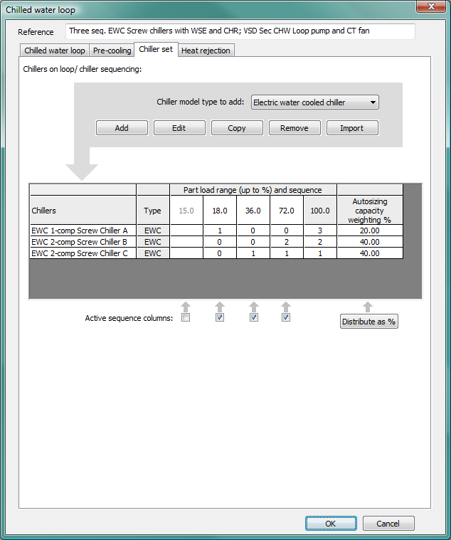
Chiller Set tab
The Chiller set tab facilitates the definition of the chillers serving the chilled water loop. Chillers can be added, edited, copied and removed from the existing chiller list (shown in the first column of the chiller sequencing table, see below) using the corresponding buttons. Chillers can also be imported from an existing chilled water loop using the Import button.
A chiller-sequencing table is provided to set the order in which chillers are turned on within any particular load range and to set the relative weighting of autosized capacities. Tick boxes are provided to activate up to 5 load ranges for sequencing and the cells with white background can be edited by double clicking. The cells containing chiller names in the Chiller list column provide access to editing individual chillers.
Figure 3 - 72 : Chiller set tab in Chilled water loop dialog.
Chiller sequencing example
Load range: 20% 40% 60% 80% 100% Autosizing capacity weighting (%)
Chiller A - 1 1 1 1 40%
Chiller B - - - 1 1 40%
Chiller C 1 - 2 - 2 20%
In the last column, Chiller autosizing capacity weighting values indicate the relative proportion of the chilled water loop load that each chiller will take during autosizing.
This example will size and sequence the chillers in the set as follows:
· Chillers A and B will each have twice the autosized capacity of Chiller C.
· At less than 20% of design load, only Chiller C operates.
· Between 20% and 40% of design load, only Chiller A operates.
· From 40% to 60% of design load, Chiller C switches in as required to supplement Chiller A.
· From 60% to 80% of design load, Chillers A and B share the load in proportion to their share of the overall design capacity (indicated in the 100% column).
· Above 80% of design load, Chillers A and B initially share the load in proportion to their design capacities, with Chiller C switching on to top up as necessary.
In this example, Chiller C is a “pony chiller” sized for and operated only when loads are either very low or to supplement the two larger chillers. Above 20% of design load (presumably more common conditions), the chillers are sequenced to share the load and ideally also to optimize operating efficiency. Appropriate sequencing will depend upon the particular distribution of hours at any particular load, the part-load performance curves for selected equipment, and the intent of the operating scheme.
When the active chillers within a part-load range reach maximum output, the sequencing moves automatically to the next range, until it reaches 100%.
The example of three sequenced water-cooled chillers of two sizes shown in Figure 3-72 above, as included with the pre-defined systems, illustrates the intentional setting of load ranges that are offset with respect to the fraction of cooling capacity provided by each chiller in the set. This might be done, for example, to minimize the operation of any chiller
Up through version 6.4.0.4, any load in excess of 100% will be met by the combination of all chillers active in the 100% column with operating performance held constant with respect to part-load curves. However, as of version 6.4.0.5, if the full load cannot not be met with all chillers operating a maximum output under the current outdoor conditions, etc., then the load will be underserved—i.e., the supply water temperature will be warmer than the specified setpoint for this value.
Chiller Model Type to Add
Selection made in this combo list determines the model type of the chiller to be added by clicking the chiller Add button. Currently three model types are available: part load curve chiller, electric water-cooled chiller or electric air-cooled chiller.
The chiller set can include any number of chillers or similar cooling sources defined using one of three models, and the set can include any combination of the three different model types:
· electric water-cooled chiller (uses editable pre-defined curves and other standard inputs)
· electric air-cooled chiller (uses editable pre-defined curves and other standard inputs)
· part-load-curve chiller (flexible generic inputs; can represent any device used to cool water via a matrix of load-dependent data for COP and associated usage of pumps, heat-rejection fans, etc., with the option of adding COP values for up to four outdoor DBT or WBT conditions)
Chiller List
The chiller list column lists the chillers and similar cooling sources in the chiller set for the current chilled water loop. To open the edit dialog for that chiller, double-click a chiller name on the list or select a chiller and click the Edit button.
Chiller Type
The chiller type column lists the types of the chillers defined for the chilled water loop. The chiller types are determined automatically by the program depending on the chiller model type selection when the chillers are added.
Currently there are three chiller model types available: part load curve chiller, electric Water-cooled chiller, and electric air-cooled chiller.
Part Load Range (up to %)
The part load range (%) values can be edited, with the exception of the end value (100%). Part load range values must always be non-decreasing from left to right. The number of part load ranges is currently limited to a maximum of 5.
Chiller Sequence Rank
Chiller sequence ranks are entered in the body of the table, for each chiller and for each part load range. These are integers in the range (0, 99) defining the order in which the chillers will be sequenced during simulation. Within a specific part load range, chillers with lower sequence rank will be sequenced in first. At least one chiller should have a nonzero sequencing rank in every column.
When multiple chillers are specified to have the same sequence rank for a part load range, the chillers will be sequenced in together in that part load range, and will share the loop load in proportion to their design capacities.
Within any range (except the last), if all the specified chillers are operating at maximum output, it is automatically moved to the next range.
For version 6.3, the cooling capacity of chillers is used to determine the top end of the performance curves (scaling the curves accordingly), but does not constrain output: any load exceeding the total available capacity at 100% of the design sizing cooling load will be met by the equipment sequenced ON in the 100% column using the performance values associated with the closest available point on the curves. In other words, the performance under a given set of conditions will be held constant as the capacity exceed the maximum that was determined or set for sizing purposes. In this context, constrain of capacity is determined at the cooling coil or chilled ceiling. However, in subsequent versions the capacity of chillers and similar cooling sources can be constrained, such that the cooling devices served by them can be modeled as collectively falling short of addressing the total of all coincident loads. This is useful in modeling low energy systems, such as cooling systems with a cooling tower by no chiller, designed to be just capable of meeting the full load under particular design conditions, but not all anticipated conditions.
Chiller Autosizing Capacity Weighting
Chiller autosizing capacity weighting is a column of values indicating the relative proportion of the load that each chiller will take during autosizing. If the rightmost sequence rank is zero for any chiller, the corresponding autosizing capacity weighting will be set automatically to zero. Any chiller with a zero autosizing capacity weighting will not be autosized. The ‘Distribute as %’ button normalizes the autosizing capacity weightings so that they sum to 100. When all the autosizing weightings are zero the ‘Distribute as %’ button will be disabled. It is not obligatory to use the ‘Distribute as %’ button as the values will be normalized automatically when applied.
Active Sequence Columns
Under each part load range column of the chiller sequencing table (except the 100% column), there is a checkbox indicating the current status of the column. These checkboxes can only be ticked in the order of right to left, and un-ticked from left to right.
For a new chilled water loop, the first 3 checkboxes (under the 1st three columns from the left) are initially grayed out and the checkbox immediately to the left of the rightmost part load range column (the 4th one) will have an enabled state.
When a check box is ticked, it will populate the column immediately above it with the data from the column to the right of it, thereby rendering the column immediately above it editable. Furthermore, a checkbox under a column to the left of this checkbox will be enabled simultaneously.
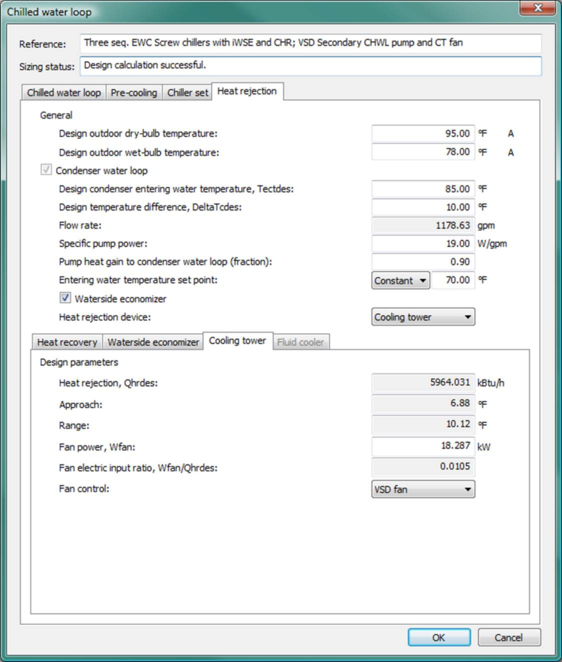
Heat Rejection tab
(updates pending – needed for changes in organization of the dialog)
The Heat rejection tab ( Figure 3-73 ) facilitates the definition of the design outdoor dry-bulb and wet-bulb temperatures for the heat rejection and for setting the parameters of a condenser water loop. The design conditions for heat rejection are used for all electric air-cooled and water-cooled chiller models and associated cooling towers. The condenser water loop in this tab functions for all water-cooled chillers in the attached chiller set and includes condenser water temperatures, cooling tower, condenser water pump, condenser hear recovery, and waterside economizer. There are now (as of VE 6.4.0.5) also options for wet and dry fluid coolers (closed-circuit towers) in place of the standard open cooling tower model. Inputs and controls for the integrated waterside economizer are located (for VE 6.4.0.x) on the Pre-cooling tab; however, as several pre-cooling options for the chilled-water return will be added in version 6.5, the integrated waterside economizer, which is tied to the cooling tower or fluid cooler on the condenser-water loop, will move to the Heat Rejection tab.
As noted below, condenser water loop flow rate is calculated from heat rejection load and condenser water temperature range at the design condition and the condenser water pump speed and flow rate are constant whenever the chiller operates. The heat rejection device (cooling tower or fluid cooler) is automatically sized for the heat rejection load at the design condition. The fan in the heat rejection device then modulates (speed if two-speed or variables-speed, otherwise on/off) in an attempt to maintain the set condenser-water loop design temperature.
If the outdoor conditions exceed the design condition, with the heat-rejection device is fully loaded, including any oversizing factor applied when sizing the associated chiller(s), the return water from the tower back to the condenser will be warmer than the design condition and the chiller model will account for this in terms of both chiller capacity and energy consumption.
If the cooling tower uses a single- or two-speed fan, results for energy consumption may still appear to vary with time, as an on/off cycling ratio will be applied to the fan power for the fan speed that is in use.
Figure 3 - 73 : Heat rejection tab in the Chilled water loop dialog with the heat rejection device set to Cooling tower.
Design Outdoor Dry-bulb Temperature
Enter the design outdoor dry-bulb temperature.
This parameter is autosizable. When this parameter is autosized, its value in the field and its autosizing label ‘A’ become green.
Design Outdoor Wet-bulb Temperature
Enter the design outdoor wet-bulb temperature for the cooling tower. This parameter is autosizable. When this parameter is autosized, its value in the field and its autosizing label ‘A’ become green.
Condenser Water Loop
When this checkbox is ticked, all of the parameters for the condenser water loop become active. There must be at least one Electric Water-cooled (EW) chiller defined for the chilled water loop.
Design Condenser Entering Water Temperature, Tectdes
Enter the design condenser entering water temperature. This design value should not be confused with the set point value below. The design value is the entering CW temperature at the design condition.
Design Condenser Water Temperature Difference ∆Tcdes
Enter the design condenser water temperature difference ∆T cdes (the difference between the condenser water leaving and entering temperatures at the design condition).
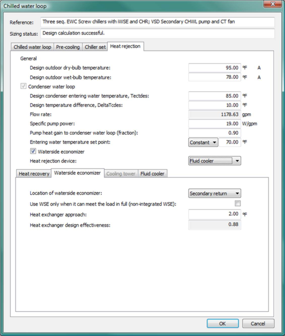
Entering Condenser Water Temperature Set Point
Entering condenser water temperature set point can be constant or set according to an absolute profile. The setpoint is typically lower than the design value at which capacity is determined.
When the condenser water temperature set point is fixed, the cooling tower or fluid cooler serving the condenser is controlled in an attempt to maintain a constant condenser water supply temperature, as limited by tower/cooler performance at off-design operating conditions.
When the waterside economizer (WSE) model is engaged and it is feasible for the WSE to meet at least some chilled-water loop load, the WSE model dynamically resets condenser loop temperature to provide WSE capacity as necessary to meet the cooling load. See details in section 3.9.6.31 Waterside Economizer.
The absolute profile option allows the flexibility of using other control strategies for the cooling tower or fluid cooler supply temperature. For example, in some applications it may be desirable to modulate the CT/FC fan (variable-speed, two-speed, or on/off, as specified by the user) to maintain a constant difference between the condenser supply water temperature and ambient wet-bulb temperature (i.e., constant approach, which may be representative of the maximum feasible capacity for any given outdoor wet-bulb temperature). As with a fixed setpoint, the profile value applies when the WSE is not operating.
The formula below is an example of using a ramp function to maintain a constant 8°F approach:
ramp (twb, 30, 38, 90, 98)
This sets CW temperature to 38° F when Outdoor wet-bulb temperature (twb) is 30°F and 98°F when Outdoor wet-bulb temperature (twb) is 90°F, with linear interpolation between these values. The upper and lower bounds should be set to reflect actual cooling tower performance and controls. This use of a condenser loop temperature profile differs from the waterside economizer (WSE) model in that the WSE model includes the ability to revert to the fixed or profiled CWL set point when WSE mode is not active.
Condenser Water Specific Pump Power at Rated Speed
Enter the condenser water specific pump power at rated speed, expressed in W/(l/s) in SI units (or W/gpm in IP units).
Condenser water pump power will be calculated on the basis of constant flow (whenever the chiller operates). The model will be based on a specific pump power parameter, with a default value of 19 W/gpm as specified in ASHRAE 90.1 G3.1.3.11.
The condenser water loop flow rate will be calculated from values of condenser water heat rejection load and condenser water temperature range through the condenser at the design condition.
Condenser Water Pump Heat Gain to Condenser Water Loop (fraction)
Enter the condenser water pump heat gain to the condenser water loop, which is the fraction of the pump motor power that ends up in the condenser water. Its value is multiplied by the condenser water pump power to get the condenser water pump heat gain, which is added to the heat rejection load of the cooling tower. (Condenser water pump is assumed to be on the supply side of the cooling tower.)
Heat rejection device
Select from the available options for heat rejection devices. Presently, these include an open cooling tower model or a closed-circuit fluid cooler. The open cooling tower model here is based on the Merkel theory, which is same as that used for the Dedicated waterside economizer component (see that section of the User Guide for details). The fluid cooler can be either wet, dry, or switch from wet to dry operation when outdoor temperature drops below a set threshold.
The fields and their labels visible when the Cooling tower option is selected are described immediately below. Changing the selection to Fluid cooler replaces these input fields with a set specific to the Fluid cooler parameters (described following the cooling tower inputs).
Cooling Tower Design Approach
This is the difference between the cooling tower leaving water temperature (T 2 ) and the outdoor wet-bulb temperature (t owb ) at the design condition. The design approach of the cooling tower is derived by the program using the provided condenser water loop design data and condenser water pump data on the Heat rejection tab, and does not need to be specified.
Cooling Tower Design Range
This is the difference between the cooling tower entering water temperature (T 1 ) and the cooling tower leaving water temperature (T 2 ) at the design condition. The design range of the cooling tower is derived by the program using the provided condenser water loop design temperature difference (delta-T c des) and condenser water pump data, and does not need to be specified.
Cooling Tower Design Heat Rejection, Qhrdes
This is the heat rejection load on the cooling tower at design condition. The design heat rejection load of the cooling tower is automatically derived by the program using the provided chilled water loop design data and condenser water pump data, and does not need to be specified.
Cooling Tower Fan Power, Wfan
Enter the power consumption of the cooling tower fan when running at full speed.
Cooling Tower Fan Electric Input Ratio, Wfan/Qhrdes
This is the ratio between the design fan power consumption and the design heat rejection load of the cooling tower. It is automatically derived by the program using the provided cooling tower fan power and the derived cooling tower design heat rejection load, and does not need to be specified.
Cooling Tower Fan control
Select the fan control type of the cooling tower. Three types of fan control are available: One-speed fan, Two-speed fan and VSD fan. When Two-speed fan is selected, you also need to specify two more parameters (see below): ‘Low-speed fan flow fraction’ and ‘Low-speed fan power fraction’.
Cooling Tower Low-speed Fan Flow Fraction
Enter the fraction of the design flow that the cooling tower fan delivers when running at low speed. This parameter only needs to be specified when ‘Fan control’ type is selected as Two-speed fan.
Cooling Tower Low-speed Fan Power Fraction
Enter the power consumed by the cooling tower fan when running at low speed, expressed as a fraction of the cooling tower design fan power. This parameter needs only to be specified when ‘Fan control’ type is selected as Two-speed fan. Generally, the low-speed power fraction will be a lesser value than the low-speed flow fraction. For example, if the low-speed flow fraction were 0.50, the low-speed power fraction would typically (depending on fan curves, motor performance, etc.) be on the order of 0.30.
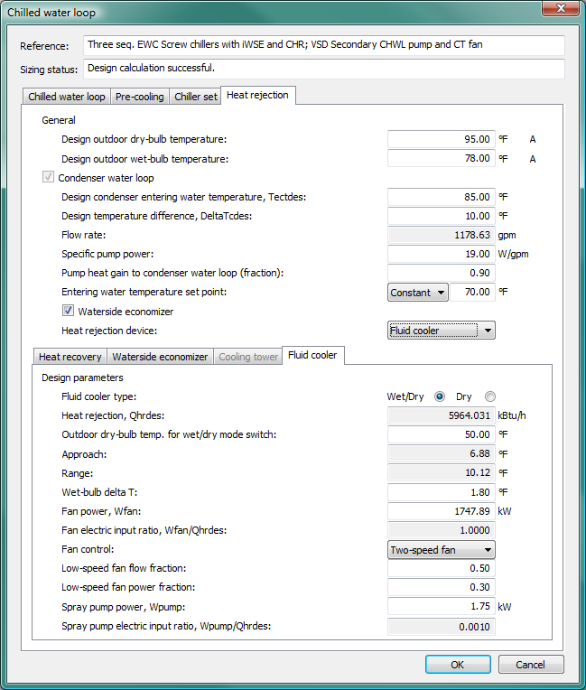
Figure 3 - 74 : Fluid cooler option selected for the heat rejection device on the Heat rejection tab of the Chilled water loop dialog.
Fluid Cooler Type
There are two types of a fluid cooler, categorised by the wetting conditions on the surface of the coil.
A dry fluid cooler is one where the coil is permanently dry—i.e., evaporative cooling is not included. This type of cooler tends to be used in areas where there are restrictions on the availability of water or where ambient conditions are particularly well suited to a dry cooler.
A wet/dry fluid cooler is one where the coil is sprayed with water to provide indirect evaporative cooling. To prevent freezing of water on the coil and/or to make the most of cool conditions, the spray pump can be switched off at low outdoor temperatures. Under these conditions the cooler operates with a dry coil.
This radio button group allows the type of fluid cooler to be selected.
Fluid Cooler Outdoor Temperature Wet/Dry Mode Switch
When a wet/dry fluid cooler has been selected this value is used to define the temperature at which the mode of the fluid cooler changes. When the outdoor dry-bulb temperature falls below the value specified, the fluid cooler will run in dry mode, the spray pump is turned off and the coil will be dry. When the outdoor dry-bulb temperature is above the value set, the spray pump will be in operation and the coil will be wet (evaporatively cooled).
Fluid Cooler Design Approach
When the fluid cooler is operating in wet/dry mode, this is the difference between the fluid cooler leaving water temperature (T 2 ) and the outdoor wet-bulb temperature (t owb ) at the design condition. In dry mode, this value is the difference between the leaving water temperature (T2) and the outdoor dry-bulb temperature (todb) at the design condition.
The design approach of the fluid cooler is automatically derived by the program using the provided chilled water loop design data and condenser water pump data, and does not need to be specified.
Fluid Cooler Design Range
This is the difference between the fluid cooler entering water temperature (T 1 ) and the fluid cooler leaving water temperature (T 2 ) at the design condition. The design range of the fluid cooler is automatically derived by the program using the provided chilled water loop design data and condenser water pump data. It does not need to be specified.
Fluid Cooler ∆T
For the fluid cooler in wet/dry mode, this is the difference between the fluid cooler exiting wet-bulb air temperature and entering wet-bulb air temperature. In dry mode this is the difference between the exiting dry-bulb air temperature and the entering dry-bulb air temperature.
Fluid Cooler Design Heat Rejection, Qhrdes
This is the heat rejection load on the fluid cooler at design condition. The design heat rejection load of the fluid cooler is automatically derived by the program using the provided chilled water loop design data and condenser water pump data, and does not need to be specified.
Fluid Cooler Fan Power, Wfan
The power consumption of the fluid cooler fan when running at full speed.
Fluid Cooler Fan Electric Input Ratio, Wfan/Qhrdes
This is the ratio between the design fan power consumption and the design heat rejection load of the fluid cooler. It is automatically derived by the program using the provided fluid cooler fan power and the derived fluid cooler design heat rejection load. It does not need to be specified.
Fluid Cooler Fan control
Select the fan control type of the cooling tower. Three types of fan control are available: One-speed fan, Two-speed fan, and variable-speed (VSD) fan. When Two-speed fan is selected, you must also specify two additional parameters (see below): ‘Low-speed fan flow fraction’ and ‘Low-speed fan power fraction’.
Fluid Cooler Low-speed Fan Flow Fraction
Enter the fraction of the design flow that the fluid cooler fan delivers when running at low speed. This parameter only needs to be specified when ‘Fan control’ type is selected as Two-speed fan.
Fluid Cooler Low-speed Fan Power Fraction
Enter the power consumed by the fluid cooler fan when running at low speed, expressed as a fraction of the fluid cooler design fan power. This parameter needs only to be specified when ‘Fan control’ type is selected as Two-speed fan. Generally, given the physics of fan performance, the low-speed fan-power fraction will be a relatively lesser value than the low-speed flow fraction. For example, if the low-speed flow fraction were 0.50, the low-speed power fraction would typically (depending on fan curves, motor performance, etc.) be on the order of 0.30.
Fluid Cooler Spray Power, Wpump
Enter the power consumption of the fluid cooler spray pump. This input needs only to be specified for a wet/dry fluid cooler.
Fluid Cooler Spray Pump Electric Input Ratio, Wpump/Qhrdes
This is the ratio between the fluid cooler pump power consumption and the design heat rejection load of the fluid cooler. It is automatically derived by the program using the provided fluid cooler spray pump power and the derived fluid cooler design heat rejection load. It does not need to be specified.
Figure 3 - 75 : Heat rejection tab of the Chilled water loop dialog with Waterside economizer sub-tab selected.
Waterside economizer
Ticking the Waterside economizer checkbox engages an integrated waterside economizer (iWSE) model. An “integrated” waterside economizer is defined as having capability for operating in parallel with one or more chillers when the waterside economizer mode is capable of some cooling on the chilled water loop, but cannot address the entire load. The WSE always shares the cooling tower or fluid cooler specified for chiller heat rejection (it does not use a separate tower or cooler). It acts in series with chillers on the chilled water loop either to pre-cool the return water to the chillers or, when its capacity is sufficient with respect to load, to address the full cooling load for the chilled water loop.
When the Use WSE only we can meet the load in full (non-integrated WSE) checkbox is ticked, the WSE will cease to operate when it cannot meet the entire load. When this box is un-ticked (the default state), the iWSE operates to serve as much chilled water loop cooling load as is feasible. When it cannot meet the full cooling load, the iWSE will pre-cool the return water to the chiller set, reducing the cooling load on the chillers so long as it can provide useful cooling.
Because the iWSE always shares the cooling tower for heat rejection with the chiller set, the condenser water flow (i.e., cooling tower flow) is apportioned between the iWSE and chiller set such that iWSE capacity is fully utilized and only remaining cooling load is placed on the chiller set. However, when the iWSE capacity falls significantly short of meeting the loads—e.g., when the outdoor wet-bulb temperature is well above the ideal for WSE operation—the limited pre-cooling effect it provides on the chilled water return will pass more load on to the chiller set, which will in turn take more of the condenser water loop flow to satisfy chiller demand for heat rejection. In other words, as outdoor conditions render the WSE less effective, the chiller set will assume the load and gradually take over the use of the cooling tower.
Condenser loop supply water temperature (SWT) control during WSE operation:
· When WSE can meet some, but not all of load (at least enough not to be displaced by chiller):
§ SWT = OA WBT + Approach (the coldest feasible leaving temperature from the CT or FC)
· When WSE can meet all of the chilled water loop load (either exactly or with capacity to spare):
§ SWT = just cold enough to meet the load, but not colder (cycling/modulating CT/FC fan)
· When chilled water loop load is too great for WSE operation under current conditions, such that one or more chillers must provide the necessary capacity and thereby displace WSE use of CT/FC:
§ SWT = Condenser loop SWT setpoint or profile on Heat rejection tab
When the user has specified WSE operation and it is feasible (whenever it can address at least some of the load), the cooling tower or fluid cooler will be operated with the target of supplying condenser loop water sufficiently cold to meet the entire chilled water loop (CHWL) load for the current time step. When the CHWL load can be fully addressed by the cooling tower or fluid cooler without need for any chiller operation, the fan for the heat-rejection device will be modulated (variable-speed, two-speed, or on/off, as specified by the user) to produce water that is only as cold as required to address the entire CHWL load. When integrated WSE operation is feasible, but conditions limit its ability to meet the full load, the heat-rejection device will operate at maximum capacity to produce the coldest water it is capable of producing under those conditions. During integrated operation such as this, it is assumed that, because the heat rejection device may be supplying water below the condenser loop SWT setpoint, flow through any operating chiller condensers will be slowed as required to ensure condenser leaving temperature within an appropriate range for maintenance of adequate refrigerant head.
During WSE operation, so long as there is no spare WSE capacity available, the control of condenser loop temperature SWT as described above will be similar to the fixed-approach setpoint profile example given in section 3.9.6.6 . The user-defined profile, however, differs from the WSE model in that it cannot gage available WSE capacity relative to CHWL load and therefore cannot revert to a fixed or profiled CWL setpoint when WSE mode is inactive because it has been displaced by chiller operation.
At least one electric water-cooled (EWC) chiller must be included in the chiller set in order for there to be a condenser water loop, and this is prerequisite to using the integrated waterside economizer, as the cooling tower for the WSE is defined as part of the condenser water heat rejection apparatus.
Location of waterside economizer
Select the location on the chilled water loop for the waterside economizer heat exchanger. The Secondary return option places the heat exchanger immediately after the loop loads. The Primary return option places the heat exchanger on the primary loop after the confluence of the secondary return and primary/secondary “common pipe” and also after the primary loop pump.
Use WSE only we can meet the load in full (non-integrated WSE)
This selection restricts operation of the WSE to simulation time steps when it can meet the entire chilled water loop cooling. If the WSE cannot meet the load in full, and therefore the chiller must be engaged, selection of this mode will force the WSE to be disengaged at that time. This is also commonly referred to as a “non-integrated” waterside economizer, as it cannot function in WSE mode when the chiller is also operating. Because the cooling tower used for the WSE is shared with the chiller set, the tower reverts to providing only chiller condenser water heat rejection (note that this is in contrast to any cooling tower dedicated to a pre-cooling function, as can be separately established on the Pre-cooling tab).
Heat exchanger approach
This parameter sets the performance of the IWSE heat exchanger at design conditions in terms of the temperature difference between the leaving water on the load side and the entering water on the source side. For example, if the source water from a cooling tower in WSE mode is 54°F and the heat exchanger being modeled is capable of cooling the chilled water return, at design conditions with respect to temperature and flow rate, down to 57°F, the approach would be 3°F.
Heat exchanger design effectiveness
This non-editable derived parameter represents the performance of the IWSE heat exchanger at design conditions in terms of an effectiveness value between 0.0 and 1.0, with 1.0 being a perfect heat exchanger. The design effectiveness value is derived from the user input for approach. During simulation, the heat exchanger model modulates the effectiveness to account for off-design conditions, including non-design water flow rates and variations in the delta-T across the heat exchanger.
Figure 3 - 76 : Heat rejection tab of the Chilled water loop dialog with Heat recovery sub-tab selected.
Condenser Heat Recovery Recipient
The condenser heat recovery recipient (in the Heat recovery sub-tab) is the heat source loop that receives the heat recovered from the chiller condenser water loop. At present, heat recovery recipient can be a generic heat source, a hot water loop, or a heat transfer loop.
If one heat source loop is specified to be the recipient of condenser heat recovery from multiple chiller condenser water loops, the heat recovered from those chiller condenser water loops will be accumulated for this heat source loop.
Note that starting from VE 2012 (VE 6.5), all heat recovery data are now displayed, edited, and stored on the recipient side. Heat recovery recipient is displayed here on the source side for user’s information only. Please see sections 2.3.3, 2.4.6, and 2.8.10 on the details of how heat recovery data can be specified or edited for the current possible heat recovery recipients respectively: generic heat source, hot water loop, or heat transfer loop.
This field is un-editable. If the condenser water loop in a chilled water loop has been specified as one of the heat recovery source of a heat recovery recipient, this field passively displays the name of the linked heat recovery recipient. If the condenser water loop has not been specified as one of the heat recovery source of any heat recovery recipient, this field displays <None>.
When copying an existing chilled water loop, if the existing chilled water loop has a condenser water loop which has been specified as one of the heat recovery source of a heat recovery recipient, and the heat recovery model used in the linked heat recovery recipient is ‘Percentage of heat rejection’ (this can happen if the heat recovery recipient is a GHS, or heat recovery recipient is a HWL/HTL and the heat recovery model selected for the HWL/HTL is ‘Percentage of heat rejection’), then the new copy of the chilled water loop will be automatically added as one of the heat recovery source of the same heat recovery recipient, with the same heat recovery source type selected (Condenser water loop) and the same corresponding heat recovery percentages as for the condenser water loop of the existing chilled water loop. In this case, the ‘Condenser heat recovery recipient’ field in the ‘Heat rejection’ tab of the new copy of chilled water loop will display the same heat recovery recipient as that displayed in the existing chilled water loop.
When copying an existing chilled water loop, if the existing chilled water loop has a condenser water loop which has been specified as one of the heat recovery source of a heat recovery recipient, but the heat recovery model used in the linked heat recovery recipient is ‘Explicit heat transfer’ (this can happen if heat recovery recipient is a HWL/HTL and the heat recovery model selected for the HWL/HTL is ‘Explicit heat transfer’), then the new copy of the chilled water loop will not be (and cannot be) added as the heat recovery source of the same heat recovery recipient. In this case, the ‘Condenser heat recovery recipient’ field in the ‘Heat rejection’ tab of the new copy of chilled water loop will be set to <None> (different from that displayed in the existing chilled water loop).