CFD Settings (Internal Simulation)
On the MicroFlo Toolbar there is an option called ‘Settings’ (

). Users can define the various settings for the simulation at any time in the modelling process here. This is available at the room level of decomposition. The various categories of this dialogue box are described below.
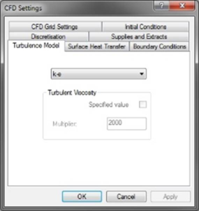
Turbulence Model
Figure 5-1: CFD Settings: Turbulence Model
There are two types of turbulence models available in MicroFlo
1. k-e (default).: This is the most generally accepted and widely used turbulence model The k-e model calculates turbulent viscosity for each grid cell throughout the calculation domain by solving two additional partial differential equations, one for turbulence kinetic energy and the other for its rate of dissipation.
2. Constant effective viscosity: This model does not attempt to account for the transport of turbulence but offers the user a much faster, much more approximate method of accounting for turbulence than the k-e model. The turbulent viscosity is assumed constant throughout the calculation domain and it can be defined either by specifying an absolute value or a multiplier, which is applied to the molecular laminar viscosity. This specification of turbulent viscosity is at best approximate but does allow a number of scenarios to be investigated for key features, prior to using the k-e model.
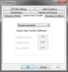
Surface Heat Transfer
Figure 5-2: CFD Settings: Surface Heat Transfer
The user has two option here:
A. Program-calculated (default): MicroFlo will calculate the heat transfer coefficient from the surface based on the local conditions of temperature and velocity around the surface.
B. User-defined: Users can explicitly define the heat transfer coefficients for various surfaces.
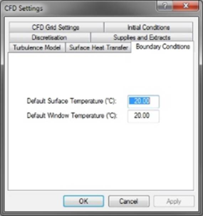
Boundary Conditions
Figure 5-3: CFD Settings: Boundary Conditions
Here you can set the default temperatures for surfaces and windows respectively. Note that doors and holes are treated as surfaces vis-à-vis these settings. These need not be set if the boundary conditions are being imported from the VistaPro results.
Grid Settings
Figure 5-4: CFD Settings: Grid Settings
This is where you define the properties of the grid.
A. Default Grid Spacing: MicroFlo will try to create the grid comprising of blocks whose each side measures this length.
B. Grid Line Merge Tolerance. The merge tolerance enables grid lines that are separated by a distance less than the tolerance to be merged into a single grid line to minimise superfluous gridding. Both values default to the last values you entered. Ensure that this value is less than or equal to the thickness of the smallest component. For example, if the walls that are imported using “Create multi-zone space partitions” are set up using 0.1m thick components so grid merge tolerance should be less than or equal to 0.1m.
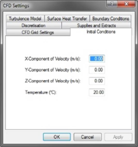
Initial Conditions
Figure 5-5: CFD Settings: Initial Conditions
The user defines the initial conditions with respect to the three velocity components and the temperature of the air before the analysis begins.
As such MicroFlo is a steady state analysis tool. So ideally, the final conditions obtained from simulation are independent of the initial conditions, However, if the flow field is set up in such a way that the initial velocity and temperature are close to the final value, quicker converge on the solution may be obtained.
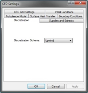
Discretisation
Figure 5-6: CFD Settings: Discretisation
This is an advanced option and is to do with the combined convection-diffusion coefficients that result from discretisation of the defining differential equation set.
Early attempts to derive CFD solution schemes using the traditional central difference approach to discretisation were found to fail for flows with high absolute value of Peclet number, due to the highly non-linear relationship between the transported variable and the transport distance.
The basic remedy for this behaviour is to allow the finite volume cell interface values of the convected properties to take on the upwind grid point values; this method is known as the ‘upwind’ scheme. Advanced users who wish to use an alternative scheme may opt for the arguably more accurate but more computationally expensive hybrid and power-law schemes.
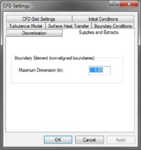
Supplies and Extracts
Figure 5-7: CFD Settings: Supplies and Extracts
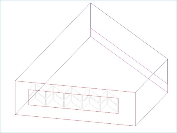
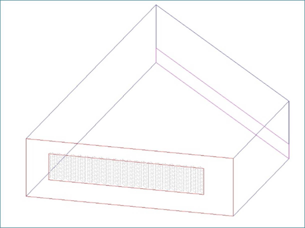
This sets the number of cell faces across a non-orthogonal inlet. This is used to determine the number of characteristic grid lines used to resolve the openings with creating the grid. Entering the command “vcomp=on” will show the inlet form. Figures 5-8 and 5-9 below show the difference in grid with different maximum dimension used.
Figure 5-8: View of non-orthogonal inlet with maximum dimension set to 1m.
Figure 5-9: View of non-orthogonal inlet with maximum dimension set to 0.25m.