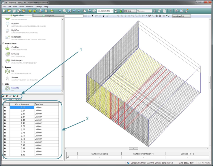
The CFD grid is the basic building blocks of the CFD model. It is the collection of small cells into which the domain is divided. Let us look first look at the CFD grid view of MicroFlo. This can be brought up by selecting ‘CFD Grid’ in the list of display modes when at room level of decomposition. CFD grid is the default view for the external simulations.
CFD Grid View
Figure 6-1: CFD Grid: Basic layout
There are two part to the basic layout of the CFD grid view.
1. Grid Manipulation Toolbar: This toolbar enables manipulation of the grid. There are 5 buttons on the toolbar
a)

: Generate Grid: Generates and/or resets grid
b)

: Insert Region: Used to insert a region between existing regions
c)

: Remove Region: Used to remove a manually inserted region
d)

: Edit Region: used to edit an existing region of the grid.
e)

: Grid Statistics: gives grid statistics
2. Grid Browser: This lists out the various regions in grid and their properties. Each region is listed by the real world coordinate of the characteristic grid line in that direction.
CFD Grid Philosophy in MicroFlo
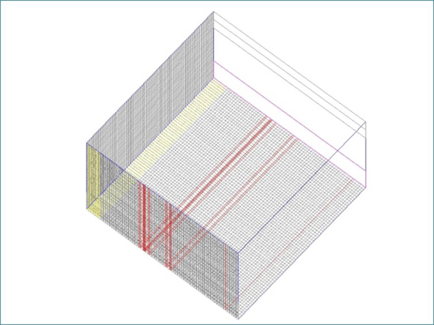
The CFD grid in MicroFlo is an orthogonal only grid. This means it is always aligned with the X, Y and Z axes of the coordinate system irrespective of the orientation of the model and/or the various surfaces in the model. The base grid is generated based on the default grid settings as supplied in
section 5.4. MicroFlo will try to create a grid that is the size of the extents of the domain and cell with sides equal to the length specified as default grid spacing. It also creates grid regions at edges of all the objects in the domain. Objects includes components, boundary conditions and rooms features likes doors and windows. This ensures that all edges and vertices of these objects are captured and that these objects are fully defined in the grid. Figure 6-2 shows how a typical grid looks likes
Figure 6-2: CFD Grid: Typical
The red lines seen are called as the characteristic grid lines. These are the lines that demarcate the region created by edges of the objects as described above. These regions are fixed and cannot be removed from the grid. These regions are also not removed even if they fall foul of the grid line merge tolerance distance.
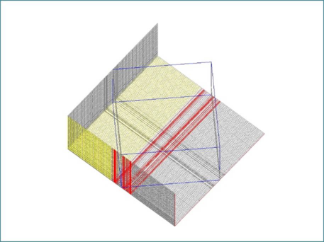
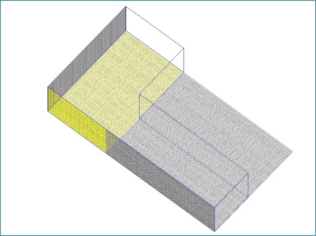
As seen above, the grid is orthogonal only. This means that for rooms not aligned with the axes or of irregular shape, the grid will extend outside the domain. Examples of this can be seen in figures 6-3 and 6-4 below.
Figure 6-3: CFD Grid: Room not aligned to orthogonal axes
Figure 6-4: CFD Grid: L-shaped room.
Grid Manipulation
The default grid generated can be modified by using the various grid manipulation techniques. These techniques are applicable to both the internal and external simulations. The commands for this can be found on the grid manipulation toolbar located on top of the grid browser as seen in figure 6-1.
Generate Grid:
This will refresh the grid based on the default grid settings as per
section 5.4 . This will also delete all the grid manipulations you have done and reset the grid to default.
Insert Region
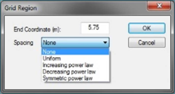
This is used to create new regions between existing regions of the grid. To insert region, select the region in the browser before which you want to insert the region. Then click on the ‘Insert Region’ button. This brings up the dialogue box shown in figure 6-5 with two user inputs
Figure 6-5: Insert Region dialogue
A. End Coordinate (m): Here the user enters the coordinate of the characteristic line that is to be introduced. This number has to be less than the region you had clicked before bringing up the dialogue box and greater than the previous number in the grid browser.
B. Spacing: This determines how the cells are distributed within the newly created region.
1. None: This create a single cell in that direction for the new region
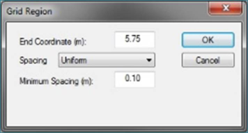
2. Uniform:
Figure 6-6: Uniform spacing
This options tries to create a uniform grid across the new region with cell length equal to the minimum spacing mentioned in this option.
3. Increasing Power Law: This option will try to create cells with lengths increasing the positive direction of that coordinate axis.
Figure 6-7: Increasing Power Law
This creates a grid in that coordinate direction in such a way that the length of the next cell is power times the length of the previous cell. The end coordinate of any cell is given by the formula:
Where,
Xi: end coordinate of the ith cell in the region (it can be Y or Z coordinate as well)
Xs: start coordinate of the first cell in the region
N: number of divisions
i: any cell in the region
power: The ratio for increase specified while defining the region.
Region length: End coordinate – Xs
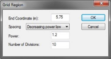
4. Decreasing power Law: This option is opposite to the previous option. Here the cell length in the positive coordinate direction goes on increasing.
Figure 6-8: Decreasing Power Law
This creates a grid in that coordinate direction in such a way that the length of the next previous cell is power times the length of the next cell. The end coordinate of any cell is given by the formula:
Where,
Xi: end coordinate of the ith cell in the region
Xs: start coordinate of the first cell in the region
N: number of divisions
i: any cell in the region
power: The ratio for increase specified while defining the region.
Region length: End coordinate – Xs
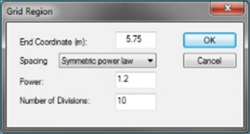
5. Symmetric Power Law: This is a combination of the previous two methods of grid size distribution where the cell size increases as per the increasing power law till the midpoint of the region and then reduces as per the decreasing power law.
Figure 6-9: Symmetric Power Law
In equation for it is written as
Where,
Xi: end coordinate of the ith cell in the region (it can be Y or Z coordinate as well)
Xs: start coordinate of the first cell in the region
N: number of divisions
i: any cell in the region
power: The ratio for increase specified while defining the region.
Region length: End coordinate – Xs
Remove Region
This command is used to remove the manually inserted regions from the grid. The default generated grid regions cannot be removed as they define the geometry of the domain.
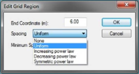
Edit Region
This command is used to edit the default and/or the manually created regions of the grid. The end coordinate cannot be edited, but the distribution can be edited. The options are same as seen in
section 6.3.2.
Figure 6-10: Edit Grid Region
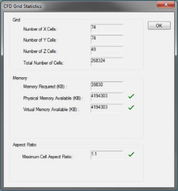
Grid Statistics
This command shows the grid statistics as per the latest grid manipulations. Figure 6-11 below shows a typical grid statistics report.
Figure 6-11: Grid Statistics
The first section gives the number of cells generated in each direction and the total number of cells in the grid. This includes the cells generated outside the zone if the zone is not rectangular and/or aligned with the coordinate axes.
The second part shows the memory details. It shows the memory required to define the grid. It also shows the memory available. This number can go up to 3.9GB of RAM only irrespective of the total memory available on your computer as MicroFlo is a 32-bit application.
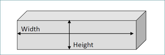
The last section reports the maximum cell aspect ratio of the grid. This is a critical parameter of the grid and health of the solution is very much linked to this parameter. Cell aspect ratio is basically the ratio of the lengths of the longest and shortest edges of any of the cells within the domain.
Figure 6-12: Cell Aspect Ratio
MicroFlo will not allow simulation to run if maximum CAR exceed 50:1. It is recommended to keep it under 10:1 for best results.