Boundary conditions can be added to the model at the surface level of decompositions. As the terminology suggests, the boundary conditions define the property of the surfaces included in the MicroFlo model. These are applicable for internal simulations only.
Boundary Condition Dialogue Box
Double clicking on a surface will give a “Boundary” view and an ‘add boundary condition’ option (

) is available on the Toolbar. Select the Toolbar and the dialogue box shown in Figure 3-1appears.
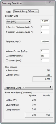
Figure 3-1: Dialogue box to define boundary conditions
There boundary condition dialogue consists of four sections
1. Type
This is a drop down box where you can select the type of boundary condition that you want to use.
The following types of boundary conditions that can be added to a surface:
a. Vent Boundaries
1. General Supply Diffuser: constant velocity inflow boundary
2. 2-Way Supply Diffuser: 2-way air supply diffuser
3. 4-Way Supply Diffuser: 4-way air supply diffuser
4. Swirl diffuser
5. Extract: constant velocity outflow boundary
6. Fixed Pressure boundary
b. Solid Boundaries
1. Fixed Temperature:
2. Heat: for convective
c. Interface Boundaries
1. Porous Baffle
2. Fan
Solid boundaries can have arbitrary polygonal geometries, but vent boundaries must be rectangular. Swirl diffusers are circular.
2. Boundary data
In this section the user inputs the various properties of the boundary that is being specified. More on this when we look at each boundary condition in detail.
3. Flow Balance
This section shows the flow balance. It lists the sum of all the various flow supplies in the row ‘In Flow’. It lists the sum of all the flow out of the domain in ‘Out Flow’ and displayed with a –ve sign. These two numbers are added together and the sum is displayed in the box underneath. If the sum is anything other than 0, the user cannot run the simulation. Flows have to balance for the simulation to take place. The user will be given an error message if the simulation is attempted.
4. Room Heat Gains
This section shows the details about the various room heat gains within the room. When the simulation is being set up as an ad-hoc simulation, the first column under title ‘Apache’ will show all zeros. This column will show non-zero numbers when boundary conditions are imported from VistaPro results. The appropriate convective part of the gain will appear under the appropriate row.
The column under ‘MicroFlo’ displays the total amount of convective gains applied manually within the domain. This is a sum of heat gains due to heat flux boundaries and components with heat source applied to them.
Drawing a boundary condition
To draw a boundary condition
1. Navigate to the surface on which you want to place the boundary condition.
2. Click on the add boundary condition’ option (
)
3. Enter all the relevant inputs in the boundary condition dialogue box.
4. Click on the surface where you want one of the corners or the first point on polygon to be.
5. Then click on the point where you want the opposite corner to be.
6. If you are drawing a polygonal boundary condition, keep clicking on points in succession to define the end points of the boundary.
7. Right click at any time to exit the boundary condition dialogue box.
8. Ensure that one boundary condition does not overlap other boundary condition or lie outside the extents of the surface.
9. If needed, the boundary condition can be moved/copied using the appropriate options on the MicroFlo Toolbar.
Vent Boundaries
These are boundaries where the flow into and out of the simulation domain is specified. Supply diffusers define the entry of air into the simulation domain. The composition can be specified, for air from an ‘external source’, such as the moisture content and the concentrations of CO2 and CO as mass fractions. The local mean age of air from any supply is defined to be zero.
General Supply Diffuser
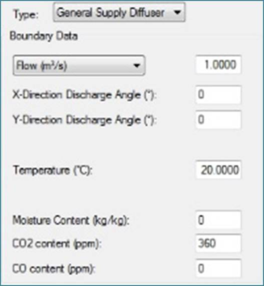
This is the simplest flow inlet boundary condition among the 6 vent boundaries. This boundary can be drawn on any surface including those which are not aligned with the co-ordinate axes. Figure 3-2 shows the properties of this boundary condition.
Figure 3-2: Inputs for General Supply Diffuser
Following inputs are required when defining a general supply diffuser
1. Flow/Velocity: Define the flow from the supply diffuser in form of either a flow rate at m3/s or a velocity normal to the plane of the diffuser.
2. X and Y discharge angles: These inputs will modify the direction away from the default normal direction. Both values can vary from -85o to +85o. The X-angle will divert the flow to the left or right, depending on whether you have specified a negative or positive angle respectively, when you are looking at that boundary at surface level. Y-angle will divert the flow in downward or upward direction based on negative or positive angle respectively. If both X and Y angles are specified, the flow will come out of the boundary at an angle which is the vector sum of the two angles specified.
Note: The velocity as seen in object properties may differ from the velocity you have specified in the dialogue box due to difference in their types. The velocity seen in object properties is the effective velocity calculated by taking into account the discharge angle specified. They will match only if discharge angles are set to zero.
3. Temperature: This is the temperature of air being supplied into the room for that boundary.
4. Moisture content: This is the amount of water vapour present in the air being supplied from that boundary. It is defined in kg of water vapour per kg of air.
5. CO2 Content: This is the amount of carbon dioxide present in the air being supplied from that boundary. It is defined in parts-per-millions of air by weight.
6. CO Content: This is the amount of carbon monoxide present in the air being supplied from that boundary. It is defined in parts-per-millions of air by weight.
2-Way Supply Diffuser
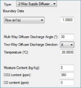
The 2-way supply diffuser allows creation of diffusers where the diffuser is automatically divided into two parts with flow diverted in opposite directions for each half. This diffuser can be drawn only on surfaces which are aligned with the co-ordinate axes. The direction of the flow will be visible in form of arrows. Figure 3-3 shows the properties of this boundary condition.
Figure 3-3: Inputs for 2-way Supply Diffuser
Following inputs are required when defining a 2-way supply diffuser
1. Flow/Velocity: Define the flow from the supply diffuser in form of either a flow rate at m3/s or a velocity normal to the plane of the diffuser.
2. Discharge angle and direction: These inputs will modify the direction away from the default normal direction. The discharge angle value can vary from 0o to 85o. The X-angle will divert the flow to the left and right when you are looking at that boundary at surface level. Y-angle will divert the flow in downward and upward direction. The flow is bent away from the normal on the line bisecting the diffuser. The bisecting line will be vertical for X-direction and horizontal for Y-direction.
Note: The velocity as seen in object properties may differ from the velocity you have specified in the dialogue box due to difference in their types. The velocity seen in object properties is the effective velocity calculated by taking into account the discharge angle specified. They will match only if discharge angles are set to zero.
3. Temperature: This is the temperature of air being supplied into the room for that boundary.
4. Moisture content: This is the amount of water vapour present in the air being supplied from that boundary. It is defined in kg of water vapour per kg of air.
5. CO2 Content: This is the amount of carbon dioxide present in the air being supplied from that boundary. It is defined in parts-per-millions of air by weight.
6. CO Content: This is the amount of carbon monoxide present in the air being supplied from that boundary. It is defined in parts-per-millions of air by weight.
4-Way Supply Diffuser
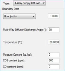
The 4-way supply diffuser allows creation of diffusers where the diffuser is automatically divided into four parts with flow diverted in opposite directions for each quarter. The division takes place along the diagonals of the diffuser. This diffuser can be drawn only on surfaces which are aligned with the co-ordinate axes. The direction of the flow will be visible in form of arrows. Figure 3-4 shows the properties of this boundary condition.
Figure 3-4: Inputs for 4-way Supply Diffuser
Following inputs are required when defining a 4-way supply diffuser
1. Flow/Velocity: Define the flow from the supply diffuser in form of either a flow rate at m3/s or a velocity normal to the plane of the diffuser.
2. Discharge angle: These inputs will modify the direction away from the default normal direction. Both values can vary from 0o to 85o.
Note: The velocity as seen in object properties may differ from the velocity you have specified in the dialogue box due to difference in their types. The velocity seen in object properties is the effective velocity calculated by taking into account the discharge angle specified. They will match only if discharge angles are set to zero.
3. Temperature: This is the temperature of air being supplied into the room for that boundary.
4. Moisture content: This is the amount of water vapour present in the air being supplied from that boundary. It is defined in kg of water vapour per kg of air.
5. CO2 Content: This is the amount of carbon dioxide present in the air being supplied from that boundary. It is defined in parts-per-millions of air by weight.
6. CO Content: This is the amount of carbon monoxide present in the air being supplied from that boundary. It is defined in parts-per-millions of air by weight.
Swirl Diffuser
A swirl diffuser creates a circular flow where the throw can be specified with respect to the radius vector. This diffuser can be drawn only on surfaces which are aligned with the co-ordinate axes. The direction of the flow will be visible in form of arrows. Figure 3-5 shows the properties of this boundary condition.
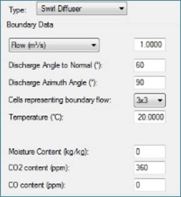
Figure 3-5: Inputs for the swirl diffuser
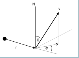
Figure 3-6: Angles for the swirl diffuser definition
1. Flow/Velocity: Define the flow from the supply diffuser in form of either a flow rate at m3/s or a velocity normal to the plane of the diffuser.
2. Discharge angle to normal: This is the angle made by the velocity vector with the normal to the surface of the diffuser drawn at the point of origin of the velocity vector. It is the angle θ in figure 3-6 above.
3. Discharge azimuth angle: This is the angle made by the projection of the velocity vector on the swirl diffuser surface and the radius vector from the centre of the diffuser to the origin of the velocity vector. It is the angle φ in the figure 3-6 above.
Note: The velocity as seen in object properties may differ from the velocity you have specified in the dialogue box due to difference in their types. The velocity seen in object properties is the effective velocity calculated by taking into account the discharge angle specified. They will match only if discharge angles are set to zero.
4. Cells representing boundary flow: As the grid in MicroFlo is castellated in nature, this enables the user to select the number of blocks that the diffuser is split into for creation of the grid. This will create the characteristic grid lines as explained in the ‘CFD Grid’ section of the user guide. The user has option to choose between “2x2”, “3x3”, “4x4” or a “5x5” The visualisation of this grid can be turned on or off by using the command ‘vcomp=on’ or ‘vcomp=off’ in the key-in command line. Swirl diffusers are generated to second order using the generated mesh and so the actual number of cells may differ from that specified.
5. Temperature: This is the temperature of air being supplied into the room for that boundary.
6. Moisture content: This is the amount of water vapour present in the air being supplied from that boundary. It is defined in kg of water vapour per kg of air.
7. CO2 Content: This is the amount of carbon dioxide present in the air being supplied from that boundary. It is defined in parts-per-millions of air by weight.
8. CO Content: This is the amount of carbon monoxide present in the air being supplied from that boundary. It is defined in parts-per-millions of air by weight.
Extract
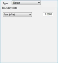
An extract boundary condition allows a fixed amount of flow to exit the domain. This boundary can be placed on surface of any orientation. Figure 3-7 shows the properties of this boundary condition.
Figure 3-7: Inputs for Extract boundary conditions
Flow/Velocity: Define the flow from the supply diffuser in form of either a flow rate at m3/s or a velocity normal to the plane of the diffuser. This is the only input required for this boundary condition.
Pressure
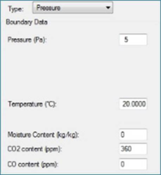
A fixed pressure boundary is a type of boundary where only the pressure and temperature of the flow is defined. Whether it acts as a supply or extract depends on the conditions in the domain. If there is more inflow than outflow, this boundary will act as an extract boundary. If the outflow exceeds the inflow, the boundary will act as an inflow. For outflow the direction of velocity at the boundary is same as that of the nearest cell. For Inflow the direction is normal to the plane of the boundary. Figure 3-8 shows the properties of this boundary.
Figure 3-8: Inputs for pressure boundary condition
1. Pressure: Pressure at the boundary in Pa.
2. Temperature: This is the temperature of air for that boundary.
3. Moisture content: This is the amount of water vapour present in the air being supplied from that boundary. It is defined in kg of water vapour per kg of air.
4. CO2 Content: This is the amount of carbon dioxide present in the air being supplied from that boundary. It is defined in parts-per-millions of air by weight.
5. CO Content: This is the amount of carbon monoxide present in the air being supplied from that boundary. It is defined in parts-per-millions of air by weight.
Solid Boundaries
Temperature
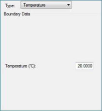
This boundary is used to assign a fixed temperature to any part of the surface within the domain. Fig 3-9 shows the properties of this boundary condition. The only input required is the temperature.
Figure 3-9: Inputs for Temperature boundary
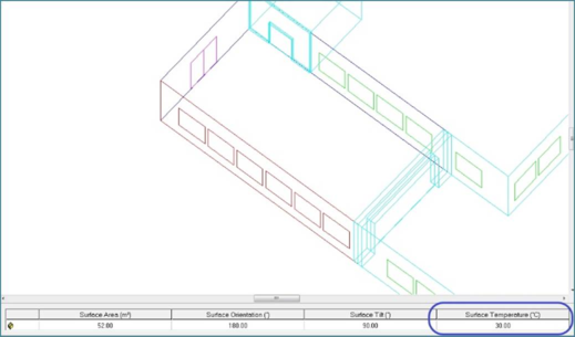
An easier way to apply lump sum temperature for wall is by changing the value by selecting any wall/ceiling/floor in the room level of decomposition and changing the temperature in the properties bar at the bottom.
Figure 3-10: Changing surface temperature
This wall change wall temperature only – not windows or doors on the wall.
Heat
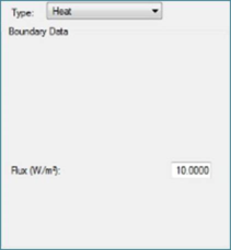
This boundary condition is used to add a heat source to the domain in form of a heat flux on the surface. The only input required is the heat flux in W/m2. The total amount of various heat sources is shown in the ‘Room Heat Gains’ part of the boundary condition dialogue box. Figure 3-11 shows the inputs for Heat boundary.
Figure 3-11: Inputs for heat boundary
Interface Boundaries
Porous Baffle
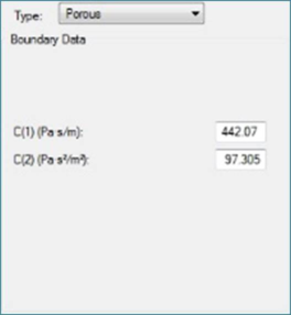
Porous baffles can only be applied to holes between two rooms which are connected to create ‘Multi-zone space’. This causes a pressure drop to the flow going across this boundary. This is similar to the effect produced by a grille or a louvre. The boundary has a symmetric behaviour, i.e. it does not matter which side the boundary is drawn on. Figure 3-12 shows the inputs for this boundary.
Figure 3-12: Inputs for Porous Baffle boundary
The pressure step for a flow of a given velocity through the baffle can be described by Darcy’s law with an inertial loss term
Or simplified as:

Where ‘a’ is the baffle thickness, ‘c’ is the pressure jump coefficient and ‘α’

is the permeability. The fluid’s viscosity and density are given by ‘μ’ and ‘ρ’. This is essentially a quadratic equation and so the simulation accepts the linear and quadratic coefficients.
The curve is cut off at the stationary point,


if c
2 is negative.
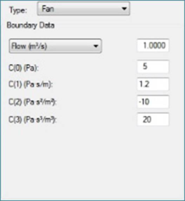
Fan
The fan interface pushes the air from one side of the hole in a multi-zone space to the other. The pressure rise due this is calculated based on a cubic fan curve. This boundary should be drawn on the side of the hole where the flow is to be ejected. The direction of the flow will be visible in form of an arrow. Figure 3-13 shows the inputs for this boundary.
Figure 3-13: Inputs for fan boundary
The cubic equation used to approximate the fan curve for a fan boundary is given as:
The user must specify a target flow rate or target velocity since there can be up to 3 solutions for the velocity for a given pressure step. Any value can in principle be chosen for the coefficients, but it is strongly recommended that a monotonic decreasing function is supplied to obtain a well behaved solution. This is one where the gradient is never greater than zero (


), and implies that

and


. A quadratic or linear function can also be given.
Set the coefficients to zero and set a target velocity if a constant velocity is required, independent of pressure.