Overview
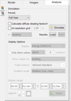
The Solar Analysis feature allows you to visually evaluate the sun intensity and exposure of your building’s façade in 3D (using Model Viewer II) over a specified time period and at a more granular level of detail if required. This can be used, for example, to assess your building for potential placement of PVs; access to sun, pedestrian comfort and landscaping. Access to this feature is through the “Analysis” tab as seen below.
There are two solar analysis options to choose from: Energy Analysis and Exposure Analysis.
These are described in more detail below.
Solar Energy Analysis

This calculation uses SunCast and Apache to generate hourly solar shading and external incident solar flux data which is then used to produce the energy results in kWh or kWh/m² for the specified period.
Calculation (for each external surface):
1. Summate the hourly solar flux values. ∑(W/m²) => Wh/m²
2. Convert the value to kWh/m². Wh/m² ÷ 1000
3. Optionally then convert the value to kWh. kWh/m² × Area
See section 5.1.3 for more info.
Solar Exposure Analysis

This calculation uses SunCast’s generated hourly solar shading data to produce the exposure results in hours and percentage of available hours for the specified period.
Calculation (for each external surface):
1. Summate the hourly percentage area values. ∑(% area) => Hours
2. Optionally then convert the value to % available. (Hours ÷ Available Hours) × 100
See section 5.1.3 for more info.
Methodology Notes
There are some general points to note when using the Solar Analysis feature. These are listed below:
· Results are only produced for the external surfaces of Spaces and (as of VE 2017) Free-standing PV Panels.
Internal surfaces and other geometry types such as Adjacent Buildings, Topographical Shades, Local Shades and so on do not produce results but will still affect the shading results produced.
· External surfaces of Spaces include: walls, roofs, windows and doors but not floors.
Please note results for doors are only calculated as part of Energy analysis.
· As with normal SunCast calculations, a single design day is used for each month.
This result is then used for every day of the month.
The design day for Solar Analysis is set to the 15th of each month.
Please note Apache still produces results for each and every day as normal.
· For each hour the sun is considered either up or down for that hour.
The exact sun up/down time isn’t taken into account.
· The SunCast surface results returned are for ‘Percentage Area’.
Percentage Area = Area In Sun ÷ Total Surface Area. See section 10.1 for more details.
· The Apache surface results returned are for ‘Ext surface incident solar flux’.
· The results displayed are an accumulation of the hourly results for the display period specified.
As the results output from SunCast/Apache are on the hour, the accumulation of results is inclusive of the start and end time, i.e. the number of results = (end − start) + 1.
For example: A single day analysis between 0800 and 1800 is the accumulation of 11 results.
Other Notes
When viewing results in Model Viewer II, please be aware that turning shadows on will apply lighting/shading to the model and therefore affect the false colours shown. This means you may not be able to match up the surface colours with the legend colours accurately.
Energy Analysis - Model Viewer II, like SunCast, does not take into account daylight savings time (DST), so please be aware of this when viewing shadows on your model during the DST shift.
Please note Apache does produce results which take into account DST.
Simulation Setup
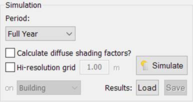
Setting up your simulation is easy and comes with a range of options as seen below.
The first option lets you choose your desired simulation period. This can be a full year, a single month, a single day, or a specific date range.
The next option is whether or not you want to take into account diffuse shading factors when running your simulation. This will make your Energy Analysis results more accurate however, it comes at the cost of increasing your simulation time. The Exposure Analysis is not affected by this output but the option is still there in case you want to then go on and perform Energy Analysis.
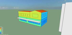
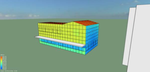
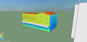
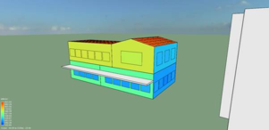
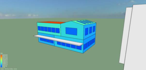
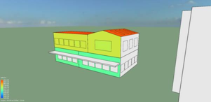
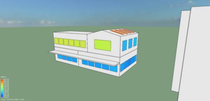
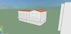
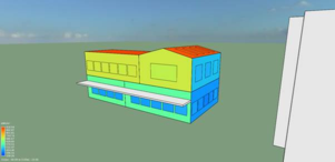
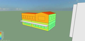
The last option allows you to get a more detailed analysis and visual result by slicing up your building’s façade into square metre (or square feet) grid cells. Again this option comes at the cost of increasing your simulation time. Below is an example with the ‘hi-resolution grid’ option turned off and on respectively. As of VE2016 you can choose to slice up your whole building (as before), just the walls, or just the roofs.
Once results have been generated they can be saved and opened again later (see section 5.4).
Display Setup
When you have results to work with you can then view them in Model Viewer II.
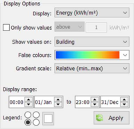
There are various options to change what and how you visualize you results.
The first option allows you to select what values you want to apply to your model and depends on the analysis performed, for example in kWh/m² or kWh.
The second option allows to you to filter results by only applying colour to surfaces that: have values above or below a certain threshold; or have values within or outside a certain range. This could possibly be used to easily identify ‘hot’ or ‘cold’ spots on the façade of your building. For example:
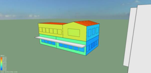
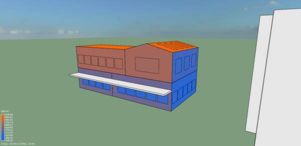
The third option allows you to only apply colours to certain types of surfaces on your model. You can choose from: everything; building only; walls only; windows only; roofs only; doors only; or PV panels only. See below:
The fourth option lets you choose what colour scale is applied to the model.
There are 13 colour scales in the list to choose from as standard.
|
Infrared Standard
|
|
|
Infrared Cold
|
|
|
Infrared Warm
|
|
|
Infrared Hot
|
|
|
Spectrum Full
|
|
|
Spectrum Part
|
|
|
Spectrum Cold
|
|
|
Spectrum Mid
|
|
|
Spectrum Warm
|
|
|
Spectrum Hot
|
|
|
Mono Brown
|
|
|
Mono Sepia
|
|
|
Mono Blue
|
|
You can add to this list by creating your own colour scales. You can add to this list by creating your own colour scales. These should be in bitmap image format (.bmp; 24bit; 512x1px), and added to the <VE>’s Shared Content directory under the ‘Texture/GradientMaps’ folder. For example:
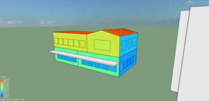
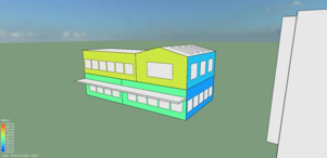
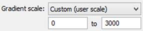
The fifth option allows you to change how each surface value is scaled in order to determine the final output colour. The three options are ‘Relative’ and ‘Absolute’ and ‘Custom’. The colours are calculated as follows:
Relative [min..max] ( value − minimum ) ÷ ( maximum − minimum )
Absolute [0..max] ( value ÷ maximum )
Custom* [min..max] ( value − minimum ) ÷ ( maximum − minimum )
The difference is shown below:
And finally the last option is the display range allowing you to change cumulative value applied to the model. The range can be anything within the simulated range.
As of VE2016 you can also change the position and colour of the legend to better suit your needs. It can be placed in one of four positions: bottom left (default), top left, bottom right and top right. Any colour can be chosen for the text; the default is white.
Once you have setup your display options, click ‘Apply’ to bring up / update your model in the viewer.
Results Persistence
As performing the Solar Analysis simulations can be time consuming you have the ability to save the results out to (a cab) file and load them back in again for future reference.
Load
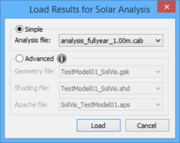
When loading in previous results for Solar Analysis you will be presented with the dialog below which gives you two options - Simple and Advanced.
Simple mode:
This option will list all cab files under your current project’s ‘SunCast/Analysis’ folder. These cab files are generated by the Solar Analysis save feature (see section 5.4.2 for more details). Simply selected the cab file you want to load and click OK. This will load in the results and display the model contained within the cab file.
Advanced mode:
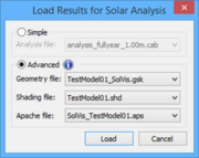
This option allows you to specify, separately, the Geometry (.gsk), the Shading (.shd), and Apache (.aps) files to apply. The Geometry files listed (if any) will be all the ones under the ‘SunCast’ subfolder that were created using the ‘
Export GSK file’ option in the SunCast menu. The Shading files listed (if any) will be all the ones under the ‘SunCast’ project subfolder. The Apache files listed (if any) will be all the ones under the ‘Vista’ project subfolder that contain ‘External incident solar flux’ data. (Please refer to the Apache Simulation > Output Options documentation for more details.) Using this option is not recommended unless you know what you’re doing, and is mainly for when you haven’t run Solar Analysis before but have results you could use. Once you have selected the Shading and Apache files you want to load, basic checks will be performed on the files - against the model and each other - to see if they can be used. Please note, due to the simplicity of the checks, it is possible that invalid data could be applied to your model. You should always try to use the Solar Analysis save feature and load the results back in from the cab file as they’re guaranteed to match the model.
Once you have loaded the results, you can then go and visualize them as normal. The UI will be marked as below indicating you are using loaded results/model to avoid any confusion.
Please note if you make any changes to the simulation options and hit ‘Simulate’ the loaded results (and model) will be wiped and your current model will be used to perform the analysis calculations as normal. Unfortunately there is no way to make changes to the previously loaded results/model.
Save
Once a simulation has been run you can save the analysis results for later investigation.
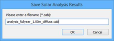
Upon clicking the ‘Save’ button you will be presented with the dialog below:
This allows you to specify the name of the cab file. The location of the cab file is fixed to the ‘SunCast/Analysis’ subfolder of your project.
Results are saved as encrypted cab files (to protect against tampering) containing the SunCast and Apache results, as well as a copy of your model in its current state. This allows you to load the model back into the VE regardless of whether the actual model has changed since saving the results.