What is CFD?
Computational Fluid Dynamics (CFD) is concerned with the numerical simulation of fluid flow and heat transfer processes. The objective of CFD applied to buildings is to provide the designer with a tool that enables them to gain greater understanding of the likely air flow and heat transfer processes occurring within and around building spaces given specified boundary conditions which may include the effects of climate, internal energy sources and HVAC systems.
The mathematical simulation of air flow and heat transfer processes involves the numerical solution of a set of coupled, non-linear, second-order, partial differential equations. MicroFlo uses the primitive variable approach, which requires the solution of the three velocity component momentum equations together with equations for pressure and temperature, these equations being known as conservation equations.
The numerical solution is conducted through the linearization and discretisation of the conservation equation set, which requires the sub-division of the calculation domain into a number of non-overlapping contiguous finite volumes over each of which the conservation equations are expressed in the form of linear algebraic equations, this set of finite volumes is referred to as a grid. The resulting linear algebraic equation set for the entire domain is then solved in an iterative scheme, which accounts for the non-linear coupling. The finer the finite volume grid, the closer the solution of the algebraic equations will represent the original differential equations but the longer the simulation will take.
In summary CFD involves the numerical solution of the following governing equations:
The benefits of using CFD include:
-
CFD is an excellent tool for ‘what-if’ analysis as once a model is created; only the setup has to be changed to try a variety of scenarios.
-
This method is quite cheaper than wind tunnel testing or other similar experimental methods. Experimental testing also brings in need to store large physical models which occupy lot of space and cannot be stored for a long time.
-
Since the models are created on computers, full size models can be created and tested without having to worry about scaling of results. Plus then can be stored for a length of the time and accessed later as needed.
-
With experimental methods, there is limit to the number of measurement sensors you can put in the space without affecting the flow. A CFD model has not such limitations and full insight in the domain is possible.
-
Time of analysis is only limited by computational power available and is usually much quicker than experimental methods.
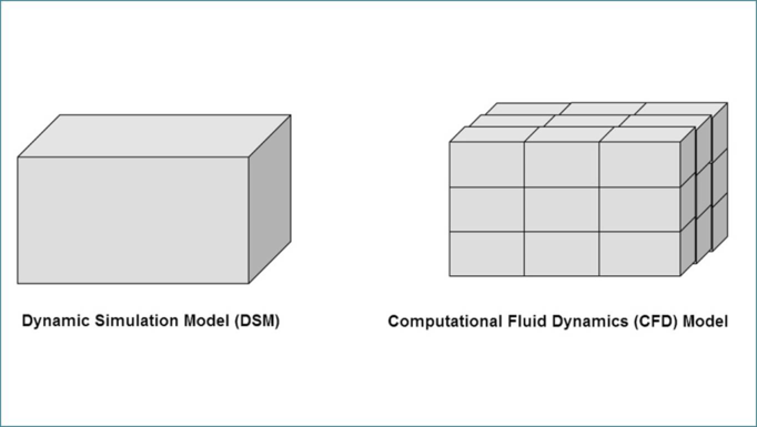
CFD in complement to Dynamic Simulation Model (DSM)
Figure 1-1: DSM v/s CFD Model
Dynamic simulation is a macro level calculation tool and assumes a fully mixed condition within a space which generates only one number for any variable within said space. This technique is fully valid for rooms which are of typical office/residential sizes without very high ceiling levels
But in conditions like high ceilings (atriums, theatre, auditorium, sports), long spaces (open plan offices, airport lounges) or concentrated large heat gains (factory shop floors, datacentres), the results generated by the DSM may not be able to paint a true picture of the conditions within such spaces. A DSM will output the average value of the quantities being measured, but in reality the range of values may be large depending on where the measurement point is. CFD compliments in such a situation being able to determine the variation in conditions across such spaces and shows a more detailed representation of conditions prevalent for those output conditions.
The best approach is using the DSM to determine the boundary conditions like surface temperatures, estimating the various heat gains/losses, flow rates through natural ventilation openings and amount of heating or cooling required under different conditions. This allows us to take into account the variations in gains and external conditions for the CFD model. The CFD model is then populated using these values and provides a deeper insight into the conditions across the domain being analysed.
Steps for CFD Analysis
The main steps involved in a CFD analysis are as follows:
Stage 1: Pre-processing Stage – Definition of the Problem
· Define the model geometry
At this stage all the various elements of the geometry are created. E.g. the model of a building will be created
· Define the computational domain.
The region for which CFD analysis is required is marked off. E.g. you could select one of the rooms or a few connected rooms.
· Define the boundary and initial conditions.
The surface temperatures and flow rates are assigned. Appropriate initial conditions are input.
· Define the grid / mesh.
The domain is divided into small blocks over which the computational equations are applied. This division is based on the type of flow expected and the size of geometry involved.
· Define all the necessary solver parameters.
Here the user chooses the computational models that are required based on expected conditions of the flow.
Stage 2: Solution Stage – Solving the Governing Equations
· Inspect the progress of the run.
Once the simulation is setup in stage 1, it is submitted to the computer for solving. While solving, the program will generate run-time output showing how the solution is progressing. The user monitors this output and makes decision on whether the simulation is proceeding on expected lines.
· Adjust solver parameter criteria if necessary to achieve convergence.
Many times, the solution will show values which the user is not expecting or are unrealistic. In this case, the user has to interrupt the solver and go back to stage 1 to look at the setup. Changes are made as per observations and simulation is run again. This is repeated until satisfactory outcome is achieved.
Stage 3: Post-processing Stage – Analysis of Results
· Visualisation of results and reporting
After the simulation concludes satisfactorily, the user will analyse the results and create a report. Based on the results, the user might want to go back and adjust the design to meet the set design criteria.