Heat Conduction and Storage

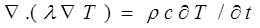
The time-evolution of the spatial temperature distribution in a solid without internal heat sources is governed by the following partial differential equations:

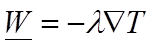
                                                                                                                 (1)

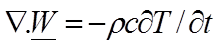
                                                                                         (2)

where

            is the temperature (ºC) in the solid at position (x,y,z) and time t

           is the heat flux vector (W/m ² ) at position (x,y,z) and time t

               is the conductivity of the solid (W/m ² K)

               is the density of the solid (kg/m ³ )

               is the specific heat capacity of the solid (J/kgK)

Equation 1 and 2 are expressions of the principles of conduction heat transfer and heat storage, respectively.

The heat diffusion equation (in its most general form in which λ, ρ, and c may vary with position) then follows:

                                                                                                 (3)

It is also necessary to consider heat storage in air masses contained within the building. The model of this process is

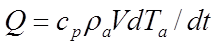
                                                                                         (4)

where

  is the net heat flow into the air mass (W)

  is the specific heat capacity of air at constant pressure (J/kgK)

is the air density (kg/m ³ )

  is the air volume (m ³ )

  is the air temperature (ºC)

 

In ApacheSim, conduction in each building element (wall, roof, ceiling, etc) is assumed to be uni-dimensional. Furthermore, the thermo-physical properties λ, ρ, and c of each layer of the element are assumed to be uniform within the layer. Under these assumptions equation 0 may be written

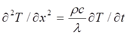
                                                                                                (5)

The system of equations is closed by the application of appropriate boundary conditions and the stipulation that W is continuous at the layer boundaries.

 

ApacheSim adopts a finite difference approach to the solution of the heat diffusion equation. This involves first replacing the element with a finite number of discrete nodes at which the temperature will be calculated.

In the spatially-discretised representation, equation 5 takes the form

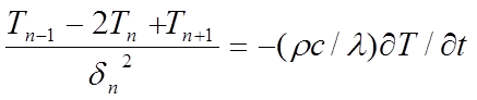
                                                                        (6)

where

  is the temperature (ºC )at node n and

  is the local node spacing (m).

 

Nodes are distributed within the layers in such a way as to ensure accurate modelling of the heat transfer and storage characteristics for the chosen time-step. This choice is based on constraints imposed on the Fourier number

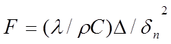
                                                                                                   (7)

where

  is the simulation time-step (s).

In this process each layer may be assigned many nodes.

Next, the time variable is discretised. A variety of schemes may be adopted for this stage.

Explicit methods use a forward-difference scheme, which uses present and future values of the nodal temperature to express the temperature time derivative at the present time:

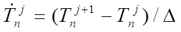
                                                                                                 (8)

where

is the temperature (ºC) at node n and time-step j,

is the time derivative of temperature (K/s) at node n and time-step j.

Pure-implicit methods use a backward-difference scheme, in which the computed time derivative is applied one time-step in the future:

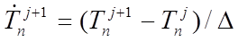
                                                                                                 ( 9)

The time derivatives in these equations are equated with  in equation to establish a model of heat conduction that is discretised in both space and time.

To improve accuracy and stability a combination of explicit and implicit time-stepping is often used. The Crank-Nicholson semi-implicit method is an example of such a scheme. Another is the ‘hopscotch’ method, which applies explicit and implicit time-stepping to alternate nodes of the construction. This is the method adopted by ApacheSim. The advantages of this method are a high level of accuracy combined with very efficient computation.

A full description of finite difference methods may be found in Myers [3].

 

Air gaps in both opaque and transparent constructions are modelled as pure resistances:

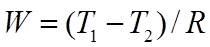
                                                                                          (10)

where

               is the heat flow across the air gap

 and     are the temperatures of the surfaces adjacent to the air gap

               is the combined radiative/convective resistance of the air gap

The value of R is set as a parameter of the air gap layer.

 

The boundary conditions for conductive elements of the building are dictated by conditions in the spaces either side of the element. These spaces may be internal or external. Where an adjacent room has been rendered inactive (for example by it being assigned in inactive layer, or not being ticked for inclusion in a <VE> Compliance analysis) the conditions on the far side are assumed to be identical to those on the near side (a reflexive boundary condition). In this way the thermal mass of the element is taken into account, while the time-averaged heat transfer through it tends to zero.

 

The dynamics of heat storage in the room air masses is described by Equation 4, in which Ta is the bulk air temperature of the room (in the stirred tank representation) and V is the room volume.

At the user’s option, the effect of heat storage in the furniture may be incorporated into the analysis. A facility is offered for modelling furniture on the assumption that its temperature closely follows that of the air. Under this assumption its effect is to increase the effective thermal mass of the air by a factor termed the furniture mass factor (f _f ). In this case, equation 4 becomes

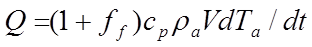
                                                                            (11)

If furniture is to be ignored, f _f should be set to 0.

In cases where the furniture has substantial thermal capacity, it is best to model it by introducing additional internal walls, with suitable thermal properties, into the room model.