Appendix F: Modeling VRF systems
While work has begun on this, the VE does not yet include an explicit model for Variable Refrigerant Flow (VRF) systems, also referred to as Variable Refrigerant Volume (VRV). The condenser heat recovery facility in ApacheHVAC, however, can be used to reasonably approximate the thermodynamic performance of such systems. This assumes that the system is configured and controlled the move heat, via a common refrigerant loop, from zones in cooling mode to those in heating mode when these modes overlap.
1. Start with a multiplexed prototype system that best represents the configuration for the actual project—e.g., PTAC, packaged single-zone, or DOAS with Fan-coil units.
2. Use a part-load-curve chiller component for the cooling mode.
The part-load-curve chiller component is used to represent the cooling mode for six reasons:
a. It has a condenser heat recovery function with which up to 100% of condenser heat can be made available for meeting heating loads.
b. It accepts connections from multiple coils (the more sophisticated DX Cooling model has one-to-one relationships between the compressor, condenser, and evaporator coil).
c. The data matrix format for part-load COP values is completely generic; this relies more on user data input, but doesn’t force the performance curve to look like a typical DX unit.
d. COP can be a single number (e.g., for a very rough model), part-load dependent, or both part-load and outdoor-temperature dependent.
e. The outdoor-temperature dependence can be DBT (it does not assume WBT as would be used for a water-cooled chiller), and irrelevant parameters for chilled water pumps, condenser water pumps, and cooling tower fans can simply be set to zero.
f. If data is available to separately account for the condenser fan peak power and power fraction associated with load on the compressor and condenser section, this can readily be included using the “Cooling tower fans” input and par-load fan-power % inputs.
Superseded by Generic Cooling Source: Note that as of version 6.3, the part-load-curve “chiller” will need to be on a “chilled water loop”; however, the water loop is readily made irrelevant by setting the W/gpm values to zero for both primary and secondary loop pumps and using the Simple cooling coil model (selected in the cooling coil dialog), which conveys load but is not sensitive to water flow and temperature. The Heat rejection tab should be left with no cooling tower. In the Chiller set, simply Add a Part-load curve chiller model.
3. Use a Generic heat source component for the heating mode.
Depending upon whether heating mode performance varies more significantly with load fraction or outdoor temperature, the part-load-curve Heating equipment inputs or Air-source heat pump (both accessed from within the Generic heat source dialog) can be used to model the heating mode (addressing heating loads when rejected heat from cooling-mode operation is not available).
In a warm climate where the variation of outdoor source temperature does not significantly influence capacity and COP, the ability to model COP variation with part-load fraction may be most valuable. Efficiency values (which can be in excess of 100%—e.g., 350% to represent a COP of 3.5) in the Part load curve heating plant dialog are used to indicate up to 10 part-load COP values. If there is backup electric resistance heating, this can be represented by a 100% efficiency value in the last (bottom) row, with the 9th data point representing the heat pump function a maximum output. There should be very small increment for the load range between the 9th and 10th data points so that the model makes a very steep transition rather than smooth ramp of the COP value between these point.
When outdoor temperature is the primary driver for heating mode performance (after using recovered heat when there is simultaneous heating and cooling), the Air-source heat pump (ASHP) may be the preferable option when outdoor temperature is the primary driver for heating mode performance (after using recovered heat when there is simultaneous heating and cooling). The reasons for this are that the ASHP model varies according to outdoor temperature (and thus thermal lift) and also has a setting for the Minimum source temperature below which the unit will cease to operate and will depend fully upon the backup heat source.
The ASHP model can still account in some respect for variation of COP with load fraction; however, this must be entered as data points on a single composite curve that indicates both the COP and heat output available for each outdoor temperature. The curve is once again represented by up to 10 data points. For each point, users need to indicate the outside-air source temperature, COP, and heat output available at that temperature. While there are benefits in accounting for variation of performance with outdoor temperature, some analysis may be required to determine appropriate part-load adjustments to the otherwise full-load COP with relatively higher outdoor source temperatures. In other words, the user must first determine how much, assuming otherwise typical operation of the building, the heating load will be reduced from the full-load condition as outdoor temperatures rise. This can then be used to adjust COP according to load fraction for data points associated warmer outdoor temperatures.
When using the ASHP, the Part load curve heating plant (see Heating equipment Edit button) within the Generic heat source dialog can be used to represent just the backup heat source. Typically this will be electric resistance heat (efficiency = 100%).
4. Distribution losses associated with refrigerant lines can be accounted for in the Heat source dialog. Airside distribution losses are better accounted for by using the Ductwork heat pickup (heat gain/loss) component on the HVAC network.
5. In the cooling source (part-load curve chiller model), you can specify COP values dependent upon both load and OA dry-bulb conditions. Set the pump and tower fan power to zero.
6. The Condenser Heat Recovery percentage in the part-load curve chiller dialog should be 100% (indicating that all of the heat extracted from zones in cooling can be rejected to zones in heating) and the CHR recipient should point to the Generic heat source you have set up for the heating mode.
7. In the Part-load curve heating plant dialog for the Generic heat source (when using this rather than the ASHP to model heating mode) COP values will be expressed as efficiency values—e.g., 350% to indicate a COP of 3.5).
8. In the Generic heat source dialog, leave the tick box for “Use water source heat pump?” unticked, as you will already have determined the electrical energy needed to extract this recovered heat on the cooling side. Set the Heating plant type to “Other heating plant” to keep energy consumption results separate from boilers or DHW heat sources, if any, in the project. The heat load will be apportioned in the following sequence:
a. Recovered heat from the part-load cooling source, to the extent it is available
b. ASHP, if used rather than a Part-load heat source
c. Part-load heat source or backup ER heat-source for ASHP, if the ASHP is used
This method can account for the benefits of moving heat from one zone to another and variation of COP with both load and outdoor temperature (it will account for the degradation of COP and heating capacity with low outdoor temperatures only if the ASHP is used for the heating mode).
· While the COP for cooling operation will, when outdoor temperature dependence is included, always be a function of both outdoor conditions and load, rather than strictly indoor conditions, as would be the case when transferring heat from one location to another in common-loop VRF/VRV system operation, this method should provide a reasonable approximation of the system performance.
· Although the CHR facility does allow for modeling energy consumption according to a COP associated with upgrading heat from a condenser loop to a heating loop (e.g., as in a WSHP), this is not necessary in this case, as the heating coils will effectively operate as the condenser for the DX cooling when heat is being transferred via CHR. There is also an input within the part-load-curve chiller dialog for the percentage of condenser heat available for recovery. When there is no heat exchanger required in the refrigerant system, and thus no exchanger effectiveness to model, and no alternate means of rejecting condenser heat when it is being routed to condenser coils that are directly heating spaces, the available CHR percentage ought to be approaching 100%. The compressor COP should account for losses associated with compressor heat rejection directly to the surrounding air. As a small amount of heat will be lost in the distribution of refrigerant to coils in heat rejection (heating) mode, an appropriate value for available CHR percentage might be on the order of 95%, depending on the system components, configuration, and installation.
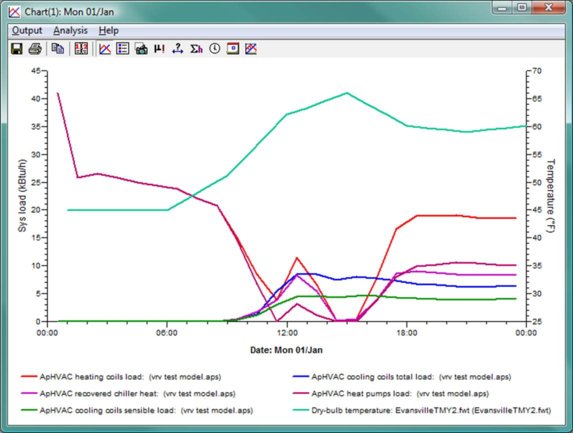
The graph below shows results for a modest 25-zone office building on a day where heating and cooling loads overlap. There is one air-source heat pump (ASHP) acting as the heating mode of the VRV system and one part-load-curve “chiller” as the cooling mode of the VRV. These components within ApacheHVAC are permitted to serve multiple heating and cooling coils, as would be the case in a VRV system.
In the illustrated example, the ASHP and part-load cooling sources are coupled to heating and cooling coils in a multiplexed stack of 25 packaged single-zone systems for the individual zones. These are created from either the prototype Packaged single-zone system 04 or prototype Packaged terminal heat pump system 02, as provided in pre-defined configuration. With just two exceptions, the pre-defined configurations remain unchanged:
· Switch the cooling coil from the dedicated DX cooling model to the part-load curve chiller model of similar characteristics set up to represent the VRV cooling mode and that includes the condenser heat recovery (CHR) capability. Set pump power in both the chiller model dialog and chilled water loop dialog to zero. This provides the capability for having many cooling coils connected to one cooling source.
o The dedicated DX Cooling model using performance curves and accounting for the entering air WBT at the DX evaporator coils provided as of VE 6.1.1 is thus far set up to run only with one DX evaporator coil per DX cooling source (compressor & condenser) and without any form of CHR to be passed to an ASHP. Therefore, the default assignment of DX coils to this model in a pre-defined system needs to be changed.
· Change the System type for the heating coils to Generic heat source and select the generic source that you have set up to represent the VRV heating mode.
o Note that as of VE 6.4.1 the ASHP is no longer placed on the airside network and has been replaced by two separate dedicated components: an air-to-air heat pump (AAHP) and air-to-water heat pump (AWHP). The former, like the DX Cooling Types, has a one-to-one relationship between the heat pump and heating coils. Therefore—until a dedicated VRV model is provided—the connection to multiple coils for a VRV model requires using the Air-source heat pump (ASHP) accessed from within the Generic heat source dialog.
The condenser heat recovery (CHR) acts as the common refrigerant loop to pass heat from the zones in cooling mode to those requiring heat. The CHR points to a Generic heat source representing the VRV heating mode (via options described above) and electric-resistance backup heat.
The ER backup is third in line to meet heating loads after the CHR and VRV heating mode (part-load-curve or ASHP) capacity are fully used. Because the backup heat source will always have an infinitely expandable capacity, any limitation of heating capacity needs to be specified in terms of the capacity of the each heating coils. Maximum cooling capacity is similarly limited by the capacity specified for each “simple” cooling coil (advanced coils, water loops, and detailed chiller models must be used to model the cooling performance of under-served coils in the case of intentionally constrained plant equipment capacity).
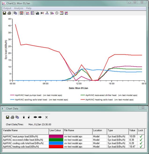
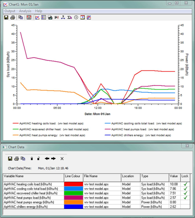
The graphs below for two different VRV examples show the recovered heat from the cooling mode (green line) taking precedence over the ASHP (VRV heating mode) to meet heating load. When energy values for the “chillers” and “heat pumps” variables are added in the second graph, these result also show that the cooling system is accounting for the energy required to extract this heat via an evaporator coil in zones where cooling is taking place and then pumping it to the heating side. Thus the electrical energy consumption for this extraction of heat from zones in cooling mode does not need to be counted separately on the heating side.
In working out the these methods, our observation is that for many building types and configurations, if the systems are suitably controlled, there should be very little temporal overlap of heating and cooling modes in a building effectively served by a large number of single-zone systems sharing a common outdoor component. It would therefore appear that, in many applications, much of the efficiency (or perhaps better referred to as efficacy) of VRV/VRF systems stems from their avoidance of the “one-size-fits-all” plus re-heat outcome typical of a multi-zone packaged VAV system. In other words, the common-loop aspect of the configuration often seems to be secondary, in terms of providing reduced energy consumption, to other aspects of VRV, such as obviating the need for re-heat.
The table of results below shows another means of confirming the transfer of recovered heat from zones in cooling mode to zones in heating mode: When there is a cooling load present and the cooling load (total for all zones presently in cooling mode) times the cooling COP—i.e., the amount of heat that needs to be rejected by the VRV system in cooling mode—is equal to or greater than the heating coils load (total for all zones presently in heating mode), then the part-load heat source or heat pump load should go to zero, as should the backup heat source if using the ASHP with backup electric heat.

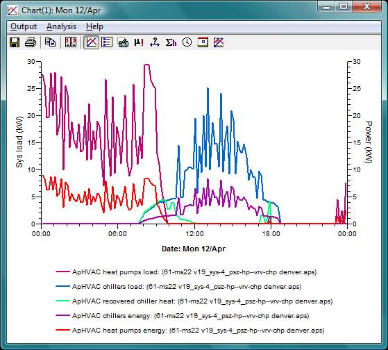
The two graphs on the next page show additional examples of results variables that can be examined to analyze the performance of VRV performance for particular project. Results such as these can be used as a quick reality check to see that the system is behaving as expects. They can also be used to provide more detailed analysis of what sort of performance might be expected under various conditions.