The output toolbar is shown below the Vista menu.
Simulation files (*.aps):
The buttons are (from left to right):
· Open File
· Results file properties
· Cursor reset
· Layer properties
· X-Y chart
· Multiple Graph Room Plotter
· Data Table
· Snapshot
· Synopsis (min\mean\max)
· Range tests
· Monthly Totals
· Comfort Settings.
· Peak time table
· Peak day table
· Peak day graph
· Peak day graph autosave
· Model Viewer
Heating Loads (*.htg):
The buttons are (from left to right):
· Open File
· Results file properties
· Cursor reset
· Layer properties
· Building and System Loads report
· X-Y chart
· Multiple Graph Room Plotter
· Data Table
· Synopsis (min\mean\max)
· Comfort Settings.
· Heating loads summary
· Radiator selection
· Model Viewer
Cooling Loads (*.clg):
The buttons are (from left to right):
· Open File
· Results file properties
· Cursor reset
· Layer properties
· X-Y chart
· Multiple Graph Room Plotter
· Data Table
· Snapshot
· Synopsis (min\mean\max)
· Range tests
· Monthly Totals
· Comfort Settings.
· Peak time table
· Peak day table
· Peak day graph
· Peak day graph autosave
· Room cooling loads summary
· Room cooling loads detail
· Air sizing summary
· System loads summary
· System loads detail
· Model Viewer
The Open File button has been described before, and is used to add sets of results. The reset cursor button acts in the same way as for ModelIT. The other buttons will generate a new chart/table and display it straight away, incorporating the currently selected variables for the currently selected parts of the building these will be explained in greater detail in later sections of this user guide.
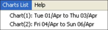
When charts or tables are created, they are listed in the Charts List menu. You can minimise a chart, and it will remain listed here. When you select it in the list it will be displayed again. If you close a chart, it is removed from the list, and completely removed from memory.
The Common Chart Dialog
The common chart dialog is used to accommodate the different displays and manipulation for the displayed output. It will appear automatically when one of the output buttons have been clicked on the Output toolbar.
The two main menu items in the common chart dialog are Output and Analysis.
Output Menu
This menu item allows you to:
|
Copy
|
Copies the current output to the Windows clipboard for pasting into another application.
|
|
Save
|
Saves the output to the relevant file format.
|
|
Print
|
Prints the display directly to a selected printer.
|
|
Report
|
Creates a HTML report when results are being viewed as a table.
|
|
Hide
|
Minimises the chart so that it can be reactivated again by selecting the chart in the chart list.
|
|
Close
|
Destroys the chart and closes the window, removing it from the chart list.
|
Analysis Menu
This menu item allows you to change analysis/display options and has the same differet options dependant on the results being viewed:
|
Set Dates
|
Changes the days (or time) over which you want to look at results
|
|
X-Y Line Graph
|
Changes the mode to an X-Y plot
|
|
Data Table
|
Changes the display to the source data, displayed in tabular format
|
|
Snapshot
|
Shows data at a specific time and date
|
|
Synopsis
|
Summarises the data, in terms of minimum value, maximum value and mean value over the currently selected period
|
|
Ranges
|
Allows you to test the data over the currently selected dates (above/below/between set values).
|
|
Monthly Totals
|
Allows you to summarise data totals over calendar months. Primarily intended for use with variables which are given in watts or kW
|
|
Peak time table
|
Identifies the peak time for the selected variable and shows any coincident variable data chosen in tabular form
|
|
Peak day table
|
Identifies the peak day for the selected variable and shows any coincident variable data chosen in tabular form
|
|
Peak day graph
|
Identifies the peak day for the selected variable and shows any coincident variable data chosen in graphical form
|
X-Y Chart
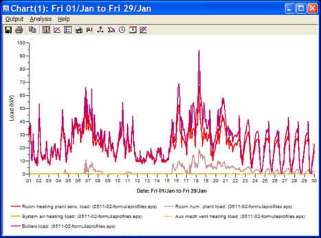
The X-Y chart mode for the common chart dialog allows you to look at a straightforward plot of the currently selected data. If you left-mouse click the graph, you can set the dates for the analysis period. Right-mouse clicking allows you to copy/save/print the graph.
If you have a large number of data selected, it is recommended that you enlarge the window (which will resize automatically) to improve the area within which the graph can be plotted.
Multiple Room Graph Plotter
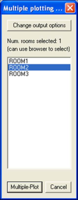
This option enables the user to automatically plot several rooms and output each graph to disk. Until the X-Y chart button is selected then this option is inactive. Once the button becomes active, we can then click the button which will execute the dialogue below:
The user can select any number of rooms from the list of rooms provided (or from the room browser) and then click the button labeled Multiple-Plot. Once clicked, a graph for each room would be saved in an enhanced meta file (*.emf) format which can easily be inserted to any reporting documentation.
Note Enhanced Meta File is a common vector based graphics format which can be easily imported into most word processors, such as: MS Word, Open Office etc.
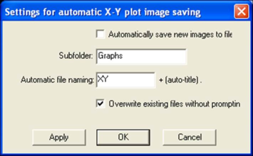
By default, each file will be saved into a sub-folder of the <project>\Vista\ folder called graphs and each file name will be pre-ceded with XY. Should you wish to change these values then click the button labeled Change Output Options which will execute the settings for automatic X–Y plot image and saving window allowing you to customise these values:
Note this window can also be executed from the menu item Settings > Automatic Graph Saving
Data Table
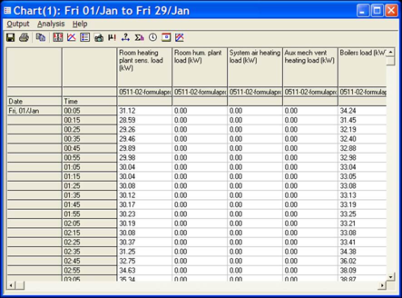
This tabular mode allows you to inspect all of the constituent data for the current selections of file, model item and variable. You can use the Output menu to Copy, Save, Print, etc. You can copy the data to the clipboard and paste it into a spreadsheet package, which should automatically drop the data into row/column formats for further analysis. The Analysis > Set Dates menu can also be used to change the analysis period.
If you have quite a few columns in the table, it is recommended that you enlarge the table manually to improve the appearance of what can be viewed.
Snapshot
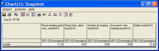
This tabular mode shows the value of any selected variable for the date/time specified:
The output can be copied, saved, etc. in the normal way, using the Output menu.
Synopsis (min/mean/max)
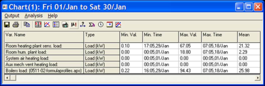
This tabular mode does a quick analysis of the selected data in terms of minimum, mean and maximum values, over the currently selected time period. The times at which the limits are reached are displayed as well.
The output can be copied, saved, etc. in the normal way, using the Output menu.
Range Tests
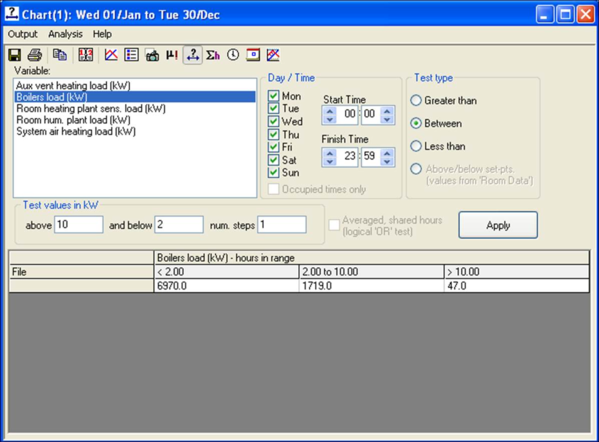
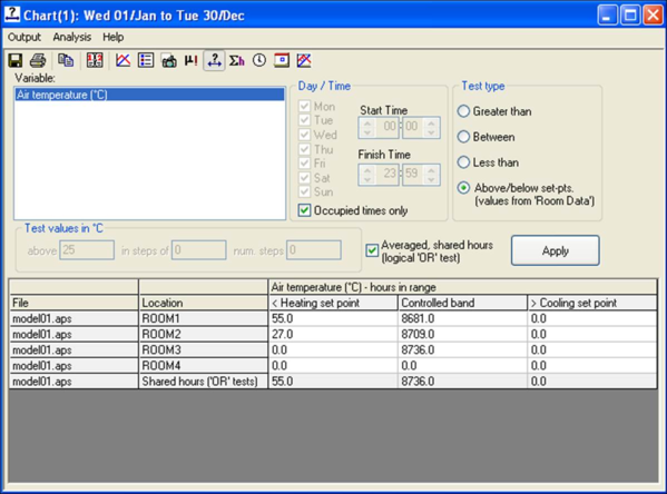
The range test mode is particularly useful if you want to test for certain conditions being met in the room of a building. It allows you to test how frequently certain limits are exceeded. The following areas of this dialog are of particular importance:
|
Variable
|
Allows you to pick the single variable to be tested.
|
|
Test Type
|
Allows you to select how the test is to be carried out (above certain values, below certain values, or between set limits).
‘Above/below set points’ tests against the room heating and cooling set points as defined in Room Conditions of the thermal template.
|
|
Values
|
Specifies the limits to be used. The number of steps specifies the number of equal graduations to be used between the specified limits.
|
|
Day/Time
|
Specifies which week days are to be tested within the currently selected period and also which times of day are to be included.
‘Occupied times only’ restricts the test to only times when there are people in the room as defined by Occupancy gains in thermal template.
|
Average, Shared hours (logical ‘OR’ test)
When the average, shared hours checkbox is ticked an additional row is added to the bottom of the table displaying the sum of hours when at least one room in the selection meets the range condition for each column.
Whenever you change the Variable selection, the table at the bottom of the dialog will be updated automatically. However, for other parts of the dialog, you will need to click the apply button to update the range test table.
Note: Above/below set points, Occupied Hours only and Averaged, Shared hours only available for room variables.
If you select more than 2 or 3 steps for the tests, then you may want to enlarge the window to ensure that all the text is visible.
Monthly Totals
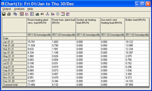
This mode for the common chart dialog will total all data values over a calendar month, based on the simulation time step (default 1 hour). It is primarily intended to total energy and load values as kWh values, allowing power demand and usage to be analysed for the building elements.
If several variables are selected, you may need to enlarge the window to allow you to see all of the text.
Set Dates
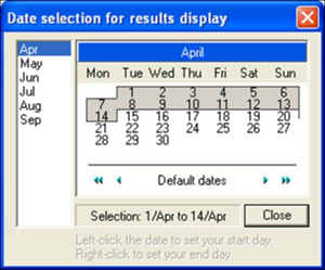
The Set Dates dialog is used to set the start and finish dates for viewing in the common chart dialog.
In the main month area of the dialog, if you left-mouse click a day, then that day will be set as the start day to view. You can right-mouse click a day to set that day as the end-day. Move between months using the list at the left of the dialog. All currently selected days are displayed with a grey background.
Click Default Dates to select the entire simulation period.
Click the blue single arrow (backwards or forwards) to move the whole selected period by the same duration as the span between the start and end days. That is, if you select 7 days of a month, and you click the Next Selection single arrow button, then the selection will be moved forwards one week. If you select a whole calendar month, and click the same button, then it will move the whole selection one month forward.
Click the blue double arrow (backwards or forwards) to skip to the corresponding month, in order to make a selection.
Any changes in this dialog will be immediately reflected in the associated common chart dialog which is displayed at the time.
In the case of a Snapshot the date is taken to be the
Comfort
Comfort Settings
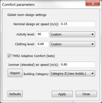
By selecting the comfort settings button on the Vista toolbar, the user is presented with the dialog below, enabling them to define their comfort parameters. By default, the comfort settings are initialised to sensible values.
From the drop down list provided, the user may choose from a pre-defined list or opt to enter a customised value. Once the user is happy with their new settings, simply click the Apply button to change the current settings/parameters.
Tick the TM52 Adaptive Comfort checkbox to access the inputs for assessing adaptive thermal comfort in line with CIBSE TM52 2013. This is required before the applicable variables will be displayed in VistaPro, please refer to the VistaPro Adaptive Thermal Comfort (CIBSE TM52) User Guide for further details.
Peak Time Table
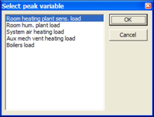
The peak time table takes a variable and shows produces a table that shows the peak time of the peak value of that variable. Firstly the variables have to be selected, this is done from the variables list, then after selecting the peak time table button a dialog appears:
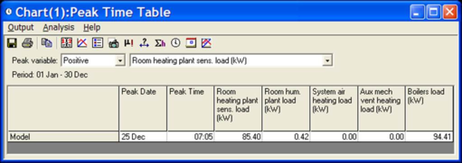
Once the peak variable has been selected the peak time table is shown as below:
The drop down list at the top of the peak time table will change the peak variable.
Peak Day Table
The peak day table takes a variable and shows produces a table that shows the peak day of the peak value of that variable. Firstly the variables have to be selected, this is done from the variables list, then after selecting the peak day table button a dialog appears:
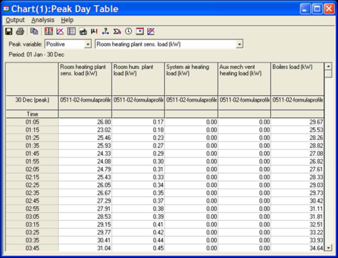
Once the peak variable has been selected the peak day table is shown as below:
The drop down list at the top of the peak day table will change the peak variable.
Peak Day Graph
The peak day graph takes a variable and shows produces a table that shows the peak day of the peak value of that variable. Firstly the variables have to be selected, this is done from the variables list, then after selecting the peak day graph button a dialog appears:
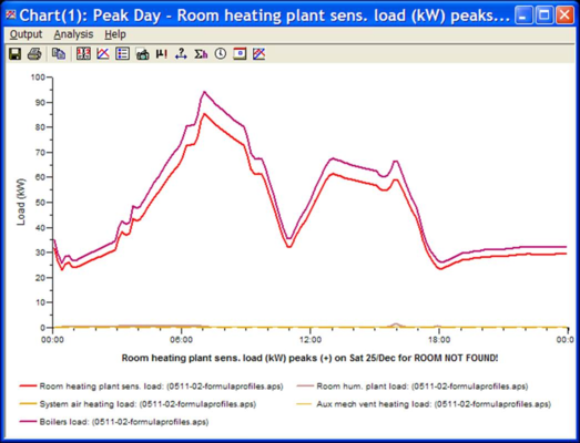
Once the peak variable has been selected the peak day graph is shown as below:
The drop down list at the top of the peak day graph will change the peak variable.
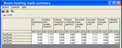
Heating Loads Summary
The heating loads summary button only appears if heat loss in ApacheCalc or heating loads in ApacheLoads. This summary identifies the heating loads and all the losses that make up the heating load on the room:
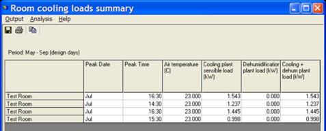
Cooling Loads Summary
The cooling loads summary button only appears if heat gains in ApacheCalc or cooling loads in ApacheLoads. This summary identifies the cooling loads and all the gains that make up the cooling load on the room:
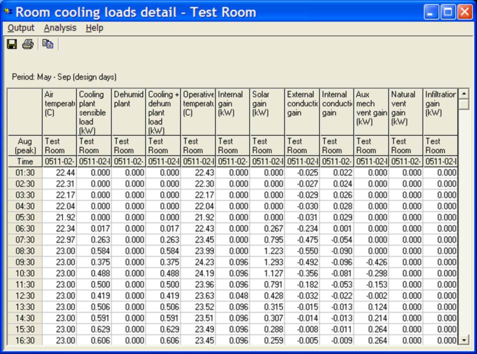
Cooling Loads Detail
The cooling loads detail button only appears if heat gains in ApacheCalc or cooling loads in ApacheLoads. This dialog identifies the cooling loads and all the gains that make up the cooling load on the room for the currently selected period.
Air Flow Sizing Summary
The air flow sizing summary button only appears if heat gains in ApacheCalc or cooling loads in ApacheLoads. This dialog identifies the air flows into all chosen rooms.
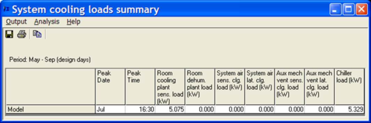
System Cooling Loads Summary
The system cooling loads summary button only appears if heat gains in ApacheCalc or cooling loads in ApacheLoads. This dialog identifies the loads on the apache system that are used in the model.
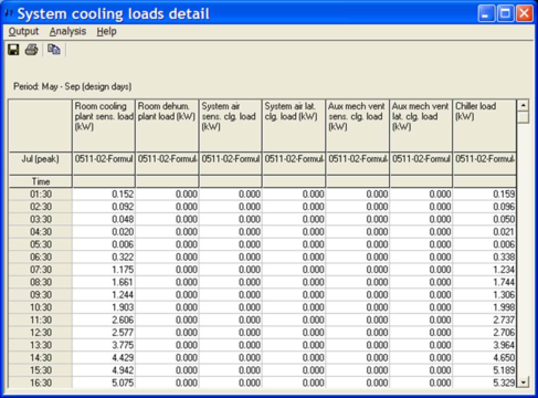
System Cooling Loads Detail
The system cooling loads detail button only appears if heat gains in ApacheCalc or cooling loads in ApacheLoads. This dialog identifies the loads on the apache system that are used in the model detailed by the current selected time step.
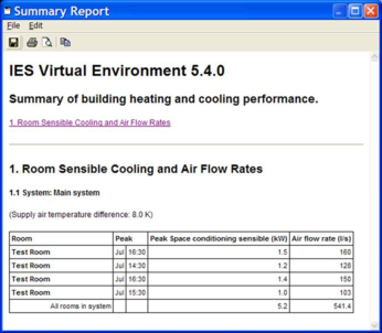
Building and System Loads Summary
This summary creates a HTML report that shows a summary of both the heat loss/heating loads and heat gains/cooling loads. An example of this output is shown below:
IES Virtual Environment 5.4.0
Summary of building heating and cooling performance.
1. General Summary
|
Model Data
|
Cooling Calculation Data
|
Heating Calculation Data
|
|
Project file: "0511-02-FormulaProfiles.mit"
|
Cooling results file: "0511-02-FormulaProfiles.clg"
|
Heating results file: "0511-02-FormulaProfiles.htg"
|
|
Model total floor area = 42.7 m²
|
Calculated at 14:49 on 03/Nov/05
|
Calculated at 14:49 on 03/Nov/05
|
|
Model total volume = 110.6 m³
|
Calc. Period: May - Sep
|
Calc. Period: January
|
|
Number of rooms = 4
|
|
|
2. Building Heating Loads Summary
|
System
|
Room load (kW)
|
Air heating load (kW)
|
Boiler load
|
|
Heating plant sens.
|
Hum. plant
|
System air
|
Aux mech vent
|
(kW)
|
(W/m²)
|
|
Main system
|
6.85
|
1.31
|
0.00
|
0.00
|
8.98
|
210.25
|
|
Auxiliary Mech Vent
|
0.00
|
0.00
|
0.00
|
0.00
|
0.00
|
n/a
|
|
Total
|
6.85
|
1.31
|
0.00
|
0.00
|
8.98
|
210.25
|
3. Room Heating Plant Loads
|
Room
|
Air temp. (C)
|
Conduction gain (kW)
|
Air system input sensible (kW)
|
Ventilation gain (kW)
|
Heating plant sensible load (kW)
|
|
External
|
Internal
|
Aux mech vent
|
Infiltration
|
Natural vent
|
|
Test Room
|
19.00
|
-0.60
|
-0.00
|
0.00
|
-1.11
|
0.00
|
0.00
|
1.71
|
|
Test Room
|
19.00
|
-0.60
|
-0.00
|
0.00
|
-1.11
|
0.00
|
0.00
|
1.71
|
|
Test Room
|
19.00
|
-0.60
|
-0.00
|
0.00
|
-1.11
|
0.00
|
0.00
|
1.71
|
|
Test Room
|
19.00
|
-0.60
|
-0.00
|
0.00
|
-1.11
|
0.00
|
0.00
|
1.71
|
4. Building Cooling Loads Summary
|
Peak
|
Room load (kW)
|
System air clg. load (kW)
|
Aux mech vent clg. load (kW)
|
Chillers load
|
|
Day
|
Date
|
Cooling plant sens.
|
Dehum. plant
|
Sens.
|
Lat.
|
Sens.
|
Lat.
|
(kW)
|
(W/m²)
|
|
Jul
|
16:30
|
5.07
|
0.00
|
0.00
|
0.00
|
0.00
|
0.00
|
5.33
|
124.81
|
5. System Cooling Loads
|
System
|
Peak
|
Room load (kW)
|
System air clg. load (kW)
|
Aux mech vent clg. load (kW)
|
Chiller load
|
|
Day
|
Date
|
Cooling plant sens.
|
Dehum. plant
|
Sens.
|
Lat.
|
Sens.
|
Lat.
|
(kW)
|
(W/m²)
|
|
Main system
|
Jul
|
16:30
|
5.07
|
0.00
|
0.00
|
0.00
|
0.00
|
0.00
|
5.33
|
124.81
|
|
Auxiliary Mech Vent
|
May
|
00:30
|
0.00
|
0.00
|
0.00
|
0.00
|
0.00
|
0.00
|
0.00
|
n/a
|
6. Room Sensible Cooling and Air Flow Rates
6.1 System: Main system
(Supply air temperature difference: 8.0 K)
|
Room
|
Peak
|
Peak Space conditioning sensible (kW)
|
Air flow rate (l/s)
|
|
Test Room
|
Jul
|
16:30
|
1.5
|
160
|
|
Test Room
|
Jul
|
14:30
|
1.2
|
128
|
|
Test Room
|
Jul
|
16:30
|
1.4
|
150
|
|
Test Room
|
Jul
|
15:30
|
1.0
|
103
|
|
All rooms in system
|
|
|
5.2
|
541.4
|
7. Room Cooling Plant Loads
|
Room
|
Peak
|
Air temp. (C)
|
Load (kW)
|
|
Day
|
Date
|
Cooling plant sensible
|
Dehumidification plant
|
Cooling + dehum plant
|
|
Test Room
|
Jul
|
16:30
|
23.00
|
1.54
|
0.00
|
1.54
|
|
Test Room
|
Jul
|
14:30
|
23.00
|
1.24
|
0.00
|
1.24
|
|
Test Room
|
Jul
|
16:30
|
23.00
|
1.44
|
0.00
|
1.44
|
|
Test Room
|
Jul
|
15:30
|
23.00
|
1.00
|
0.00
|
1.00
|