A brief introduction to iVN network modelling is provided in the workflow below. A more detailed explanation of the user interface and specific network installations is provided in subsequent sections.
· Step 1: Define buildings
Buildings are a key component of iVN models as they represent building blocks for the city model infrastructure and can have demand for (or generation of) energy. Buildings can be 3D and/or 2D and need not necessarily represent real buildings (for example, buildings could represent proposed future developments).
There are a number of ways to add buildings to a model:
i) Import an iCIM model
ii) Import a 3D building model using Open Street Map (OSM);
iii) Draw a 3D building in the 3D model view workspace; or
iv) Drag and drop a building asset from the asset library to the 2D virtual network workspace (in which case no 3D model is necessary).
· Step 2: Assign time-series data
Time-series data is the main means of specifying building energy demand or generation. The time-series data can be obtained by:
i) Importing an iCIM model that includes building time-series data (Refer to section 3.4.2.1)
ii) Importing data from iSCAN (which can be measured data or simulated data from the IES Virtual Environment) and assigning it directly to building meters; or by
iii) Importing data from the CSV import function (Refer to section 3.4.2.4)
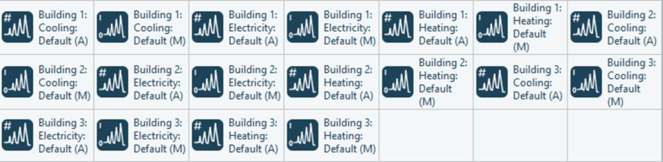
The time-series data then appears as profiles in the asset library (see Figure 2-1).
Figure 2-1: Time-series data imported from iSCAN and shown in the asset library
· Step 3: Define network objects
A 2D virtual network consist of electricity, heating, cooling, waste heat, potable water and wastewater assets (refer to section 4).
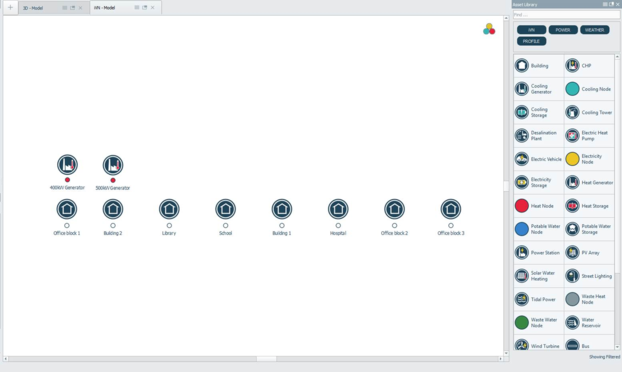
2D virtual network assets can be dragged from the asset library and dropped onto a 2D virtual network model (see Figure 2-2). Default category information can be assigned or object parameters can be manually defined.
Figure 2-2: The 2D virtual network workspace with asset library. iVN network assets are 2D buildings and nodes. Connections are established between the various assets in the next step.
· Step 4: Establish network configuration
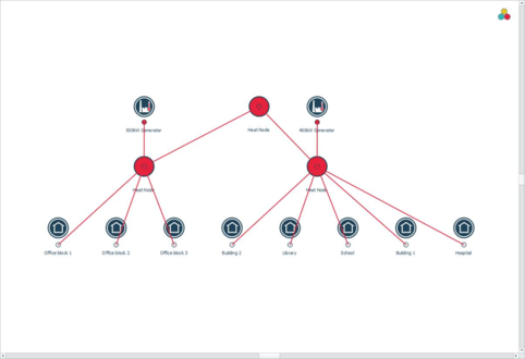
The 2D virtual network is configured by connecting all iVN assets to the nodes for the types of network which are to be simulated. The role of the network nodes is to act as decision points in a network where energy demand is aggregated and loads are allocated (to dispatchable assets), using a control strategy, in order for the providers to meet the demand. Linked nodes create a hierarchy of aggregation through parent-child relationships. An example of a configured network is shown in Figure 2-3.
Loads are allocated to attached network objects according to a control strategy, which is defined on each node. The available control strategies are (Refer to section 3.12.3):
· Balanced: allocate load evenly across all network installations, either as an absolute amount or as a percentage of maximum load;
· Ranking: allocate load in rank order except when installations have equal rank, in which case the load is balanced across those objects with equal rank.
· Sequential: allocate load in a specific order; and
Figure 2-3: An example configured iVN network. This example shows a heating network hierarchy with two nodes representing local-scale areas, “residential sector” and “commercial sector”, and a node representing a global-scale area, “root node”. The attached generators meet the demand for the buildings attached to the same node and pass their residual demand to the next node up (the root node).
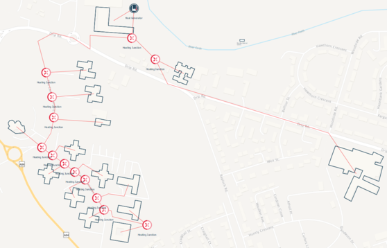
Upon the creation of a 2D virtual network users can also create a 2D physical network for heating.
A 2D physical network consists of; n(s), heat pipe(s), demand(s) and load(s). Refer to section 3.7 for further details.
Figure 2-4: Example - physical network view – Workspace
· Step 5: Network Simulation and Results
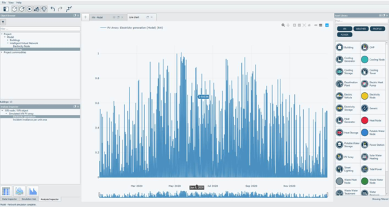
A network simulation can be performed based on the network set-up and data assigned in the previous steps. Results are then displayed in the analysis inspector and can be exported for further analysis.
Figure 2-5: Simulation results displayed in the iVN analysis inspector
· Step 6: Create scenario Models
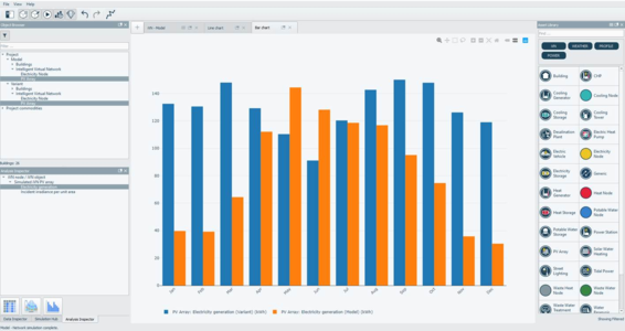
Scenario models can also be created and simulated. Scenario model results can be directly compared with the initial model results or other scenario models in order to help assess the impact of changes to the model.
Figure 2-6: PV array generation results for two scenario models shown in the iVN analysis inspector